Buried Piping
Soil in Buried piping analysis is modeled by using bilinear restraints with an initial stiffness and an ultimate load. After the ultimate load is reached, the displacement continues without any further increase in load, i.e., the yield stiffness is zero. The initial stiffness is calculated by dividing the ultimate load by the yield displacement which is assumed to be D/25 where D is the outside diameter of the pipe.
Soil modeling is based on Winkler’s soil model of infinite, closely spaced elastic springs. Soil stiffness is calculated for all three directions at each node. The pressure value in the load is suitably modified to consider the effect of static overburden soil pressure. The model is analyzed for operating (W+P1+T1) condition and the displacements in the three directions are noted. A check is made for whether skin friction is mobilized and the soil has attained the yield state. If true, then the spring is released in that direction, indicating that soil no longer offers resistance in that direction. This modified model is again analyzed and checked for the yield stage. The iterative process is continued until the percentage difference between displacements at each node for two successive iterations is less than 1%. The final stiffness is the true resistance offered by the soil to the pipe.
General Procedure to model buried piping
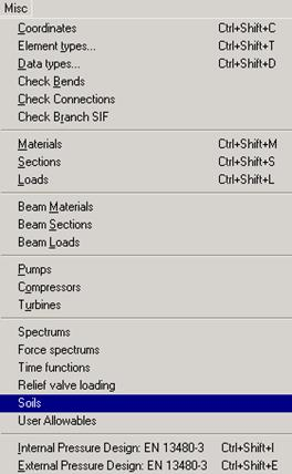
1. First, define soils using the command Misc > Soils in the Layout or List window.
2. Next, tie these defined soils with pipe sections (Ctrl+Shft+S to list Sections, double click on an empty row, you will see the field Soil in the bottom right corner. Pick the soil name from the drop-down combo box).
3. Use this modified section for each element on the Layout window that is buried with this soil around it.
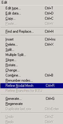
5. Discretize long sections of buried piping (Refine Nodal Mesh) through Layout window > Edit > Refine Nodal Mesh > Buried Piping.
It is at the bends, elbows, and branch connections that the highest stresses are found in buried piping subjected to thermal expansion. These stresses are due to the soil forces that bear against the transverse runs. The stresses are proportional to the amount of soil deformation at the elbows or branch connections. Hence, piping elements adjoining to bends, elbows and branch connections are to be discretized in the stress model.
In addition, to best simulate Winkler’s soil model, it is recommended to discretize even the remaining long straight buried pipe sections in the stress layout
Refinement of Nodal Mesh for Buried Piping
Modulus of Subgrade Reaction (k)
This factor k defines the resistance of the soil or backfill to pipe movement due to the bearing pressure at the pipe/soil interface. Several methods for calculating modulus of subgrade reaction (k) have been developed in recent years. As per Trautmann, C.H., and O’Rourke, T.D., “Lateral Force-Displacement Response of Buried Pipes,” Journal of Geotechnical Engineering, ASCE, Vol. 111, No. 9 Sep 1985, pp. 1077-1092, the modulus of subgrade reaction, k, can be calculated as per Eq. (2) in Appendix VII of ASME B31.1-2018 code.
where,
Ck = a dimensionless factor for estimating horizontal stiffness of compacted backfill. Ck may be estimated at 20 for loose soil, 30 for medium soil, and 80 for dense or compacted soil. In the current version of CAEPIPE, the value of Ck is internally set as 80 for both cohesive and cohesionless soil.
D = pipe outside diameter
w = soil density
Nh = a dimensionless horizontal force factor from Fig. 8 of above stated technical paper. For a typical value where the soil internal friction angle is 30 deg. the curve from Fig. 8 may be approximated by a straight line defined by
Nh = 0.285H/D + 4.3
where
H = the depth of pipe below grade at the pipe centerline
Influence Length (Lk)
The influence length is defined as the portion of a transverse pipe run which is deflected or “influenced” by pipe thermal expansion along the axis of the longitudinal run.
From Hetenyi’s theory, (Beams on Elastic Foundation, The University of Michigan Press, Ann Arbor, Michigan 1967) (also, see Section VII-3.3.2 of Appendix VII of ASME B31.1-2018 code)
where,
Pipe / Soil System Characteristics = 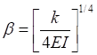
E = modulus of elasticity of pipe at reference temperature
I = moment of inertia of pipe cross section
k = modulus of subgrade reaction of soil as detailed above.
Implementation in CAEPIPE
As stated earlier, it is at the bends, elbows, and branch connections that the highest stresses are found in buried piping subjected to thermal expansion of the pipe. These stresses are due to the soil forces that bear against the transverse runs. The stresses are proportional to the amount of soil deformation at the elbows or branch connections. Hence, piping elements adjoining to bends, elbows and branch connections are to be discretized in the stress model.
In addition, to best simulate Winkler’s soil model, it is recommended to discretize even the remaining long straight buried pipe sections in the stress layout
This can be performed through Layout window > Edit > Refine Nodal Mesh > Buried Piping.
When the command is selected, CAEPIPE will refine the piping layout as detailed below.
1. Calculate modulus of subgrade reaction (k) as detailed above. While calculating k, the value of Ck is taken as 80 for both cohesive and cohesionless soil.
2. Calculate influence length (Lk) for the element that is fully buried.
3. If the length of the pipe element near bend / elbow / branch connection is greater than or equal to the influence length (Lk), then the pipe element will be split into a number of short elements with length of each short element being equal to 2 x OD of that pipe section until the Influence length (Lk).
4. On the other hand, if the length of the pipe element near bend / elbow / branch connection is less than the influence length (Lk) and greater than 2 x OD of the pipe, then the pipe element will be split into a number of short elements with length of each short element being equal to 2 x OD of that pipe section.
5. If any buried straight pipe element is longer than the influence length (Lk), then the straight pipe element will be split into a number of equal length elements, where the number of such equal length elements will be computed as [(int)(Original Straight Pipe length/Influence Length) + 1]. For example, if the total length of straight pipe element is equal to 1843” and influence length is 400”, then the straight pipe will be split into 5 equal length elements [= (int)(1843/400) + 1 = ((int)(4.61) + 1) = (4 + 1)] with each element having a length of 368.6” [= 1843/5].
Note:
While refining the layout, the new node number will be generated by adding the node increment specified (through Layout Window > Options > Node increment) to the available free node number. Hence, set the node increment value as required before refining the buried piping layout.
It is possible to specify different soil characteristics for different portions of the pipe model. Here is how.
1. Define different soils using the command Misc > Soils.
2. Associate each soil type with those sections that are buried in that soil.
3. Model the buried layout using the different sections for different buried portions.
Ground Level
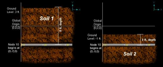
Ground level for soil is the height of the soil surface from the global origin (height could be positive or negative). It is NOT a measure of the depth of the pipe’s centerline.
In the figure, the height of the soil surface is 3 feet above the global origin. Pipe node 10 [model origin] is defined at (0,-5,0). So, the pipe is buried 8’ (3’ - [-5’]) deep into the soil. Define similarly for the other soil.
The pipe centerline is calculated by CAEPIPE from the given data
Depth of Soil above Pipe’s Centerline
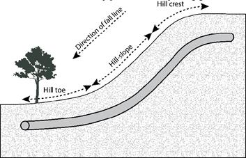
When the option “Value entered is Depth of Soil above pipe centerline” is turned ON in Soil input then CAEPIPE will compute maximum soil loads for the sections buried using the Depth entered. This option will be helpful for modeling pipes that are running up or down a hill with same depth of soil filled above pipe’s centerline as shown in the figure given below.
Warning:
Assign Soil only to those elements that are really buried in soil when the option “Value entered is Depth of Soil above pipe centerline” is turned ON.
Two Soil types
Two types of soils can be defined - Cohesive and Cohesionless. Soil density and Ground level are input for both cohesive and cohesionless soils. The Ground level is used to calculate the depth of the buried section. For cohesive soil, Strength is the un-drained cohesive strength (Cs). For cohesionless soil, Delta (d) is the angle of friction between soil and pipe, and Ks is the Coefficient of horizontal soil stress. See the nomenclature below for more information.
Highlight buried sections of the model in graphics
If your model contains sections that are above ground and buried, then you can selectively see only the buried sections of piping in CAEPIPE graphics by highlighting the section that is tied to the soil. Use the Highlight feature under the Section List window and place highlight on the buried piping section (see Highlight under List window>View menu, or press Ctrl+H). The Graphics window should highlight only that portion of the model that is using that specific section/soil.
Nomenclature
When the option “Include Insulation Thickness” in “Soil” input is turned OFF, then
D = Outside diameter of the pipe
When the option “Include Insulation Thickness” in “Soil” input is turned ON, then
D = Outside diameter of pipe + (2.0 x Insulation Thickness)
Ks = Coefficient of horizontal soil stress, which depends on the relative density and state of consolidation of soil. Ks is empirical in nature and may be estimated from Nq/50. Ks can vary depending on the compaction of the soil from 0.25 (for loose soil) to 1.0 (really compacted soil).
Nq = Bearing capacity factor = 0.98414e(0.107311f)
f = d + 5°
Normal values for delta ranges between 25° – 45° (for sand).
Clean granular sand is 30° . With a mix of silt in it, the angle is 25°
Sp = soil pressure = soil density × depth
Cs = Undrained cohesive strength (input for cohesive soil), (Cs in kN/m2) ≥1.0
Af = Adhesion factor = 1.7012775 e(-0.00833699 Cs)
kp = Coefficient of passive earth pressure
= (1 + sin f) / (1 – sin f)
bottom depth = depth + D/2
top depth = depth – D/2
Nr = (Nq – 1.0) tan (1.4 f)
dq = dr = 1.0 + 0.1 tan (p/4 + f/2) × depth / D, for d> 10° , otherwise dq = dr = 1.0
Calculation of Ultimate Loads
The ultimate loads (per unit length of pipe for axial and transverse directions and per unit projected length of pipe for vertical direction) are calculated as shown below.
Different equations are used for cohesive (clayey) and cohesionless (sandy) soils.
Calculation of Ultimate Load and Bi-linear Restraint Stiffness for all Codes other than EN13941-1
|
Buried Restraints
| ||
|
Cohesive soil
|
Cohesionless soil
|
|
|
Ultimate Axial load
|
Axial Stiffness
| |
|
|
|
Ultimate Axial load / Yield Displacement
|
|
Ultimate Lateral Load
|
Lateral Stiffness
| |
|
|
|
Ultimate Lateral load / Yield Displacement
|
|
Ultimate Vertically Downward load
|
Downward Stiffness
| |
|
|
 |
Ultimate Downward load / Yield Displacement
|
|
Ultimate Vertically Upward load
|
Upward stiffness
| |
|
|
|
Ultimate Upward load / Yield Displacement
|
After the ultimate load is reached, the displacement continues without any further increase in load, i.e., the yield stiffness is zero. The initial stiffness is calculated by dividing the ultimate load by the Yield Displacement which is assumed to be D/25 where D is the outside diameter of the pipe. This Yield Displacement is the same in all four (4) directions namely, Axial, Lateral, Vertically Downward and Vertically Upward.
When the option “Compute Lateral (Transverse) and Vertical Stiffnesses with/without Expansion Cushion as per EN 13941-1” is turned ON in Soil input dialog box, then the Lateral (Transverse) and Vertically Downward and Vertically Upward Stiffnesses are computed internally as given below for EN 13941-1.
Calculation of Ultimate Load and Bi-linear Restraint Stiffness for Code EN13941-1
Refer to the section EN13941-1 in Code Compliance Manual for details and nomenclature.
|
Buried Restraints
| ||
|
Cohesive soil
|
Cohesionless soil
|
|
|
Ultimate Axial load
|
Axial Stiffness
| |
|
|
|
Ultimate Axial load /
Ultimate Displacement
(see Note 1)
|
|
Ultimate Lateral Load
|
Lateral Stiffness
| |
|
|
|
Ultimate Lateral Load / Ultimate Displacement
(see Notes 1,2 & 3)
|
|
Ultimate Vertically Downward load
|
Downward Stiffness
| |
|
|
|
Ultimate Downward load / Ultimate Displacement
(see Notes 1,2 & 3)
|
|
Ultimate Vertically Upward load
|
Upward stiffness
| |
|
|
|
Ultimate Upward load / Ultimate Displacement
(see Notes 1,2 & 3)
|
Note 1: For details on Ultimate Displacements, refer to section titled “EN 13941-1 (2021)” in Code Compliance Manual.
Note 2: As per EN13941-1, the combined stiffness of PUR, Expansion Cushion and Soil is considered only for Lateral, Downward and Upward directions.
Note 3: The ultimate loads for Vertically Downward and Upward directions are not specified in EN13941-1 (2021). Hence, the equations listed under the Section titled “Buried Restraints for all codes other than EN 13941-1” above are used internally for computing the Ultimate Loads in Vertically Up and Vertically Downward directions.
Buried Piping Example
Ultimate Loads and Stiffnesses computed by CAEPIPE for this example are verified later in this section.
Example data:
A 12” Std pipe 6’ long is buried, 3’ in cohesionless and 3’ in cohesive soils with No Insulation properties
Soil properties are as follows:
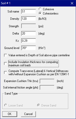
Cohesionless (Name of soil: S1, associated with pipe section 12A):
Density = 120 lbf / ft3
Delta (d) = 20°
Ks = 0.29 (calculated from Nq/50, where Nq = 14.394)
Ground level = 3’
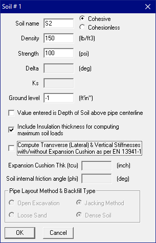
Cohesive (Name of soil: S2, associated with pipe section 12B):
Density = 150 lbf / ft3
Strength = 100 psi
Ground level = -1’
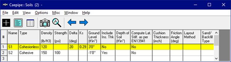
1. Define soils using the command Misc > Soils.
A List window for soils will be displayed. Double click on an empty row to define a new soil.
For our example, define two soils - one cohesionless and the other cohesive with properties as shown in the following dialogs.
Dialog for cohesionless soil:
Dialog for cohesive soil:
After you have defined the soils, you should see the two soils listed in the List window.
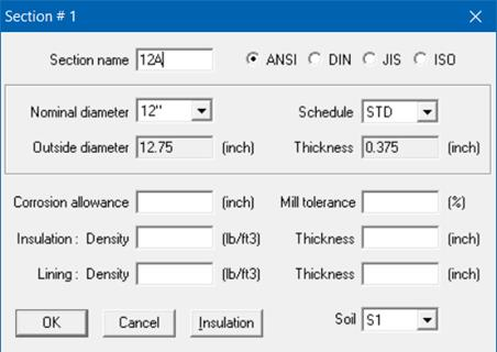
2. Define pipe sections and then associate the soils with these sections.
Define two pipe sections, both 12”/STD pipe sections (name them 12A and 12B), and select the correct soil in the pipe section dialog box using the Soil drop-down combo box.
Soil S1 is associated with section 12A:
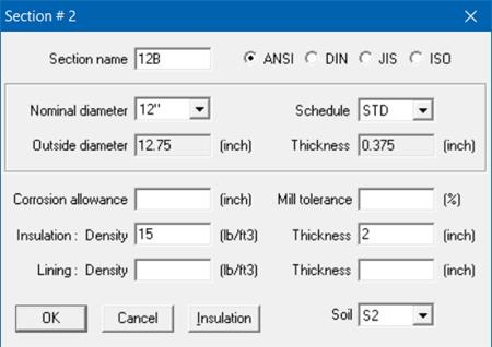
Soil S2 is associated with section 12B:
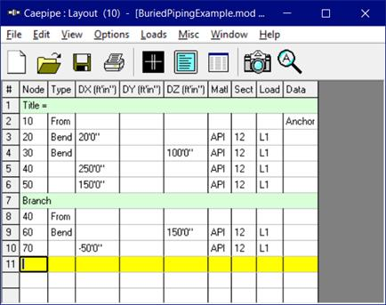
3. Define the layout from 10 to 20 to 30; the first pipe element from 10 to 20 uses section 12A (Cohesionless soil type S1), and the next pipe element 20 to 30 uses section 12B (Cohesive soil type S2). Check Operating load case under Loads menu > Load cases for analysis.
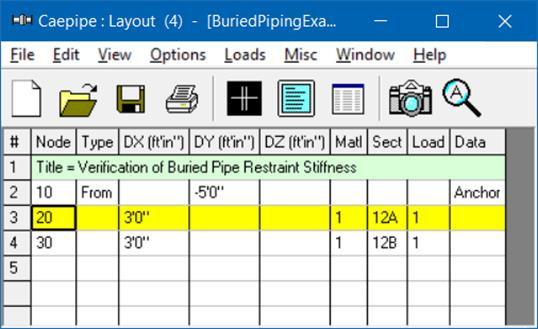
Save the model and analyze. Choose yes to view the results. From the Results dialog, pick Soil Restraints. The soil loads and soil stiffnesses in different directions as computed by CAEPIPE are now shown, which are verified below in this section.
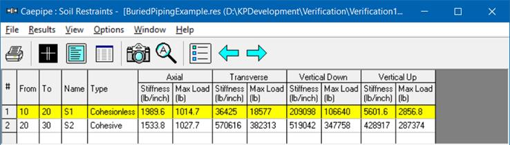
Example Verification
Verification of cohesionless restraints (for pipe element 10 to 20)
Sp = soil pressure = soil density × depth
depth = 3’ - (-5’) = 8’ (since the pipe centerline is at -5’ and ground level is at 3’).
Sp = 120 lb/ft3 × 8 ft = 960 lb / ft2 = 6.6667 lb/in2
Axial direction
Axial load = p× D × Ks × Sp × tan d
= p ×12.75×0.29×6.6667×tan (20)
= 28.1861 lb/in
= 1014.7 lb (for 36”, length of pipe) (CAEPIPE: 1014.7)
Assuming yield displacement = D/25,
Axial stiffness = 25 × 1014.7 / 12.75 = 1989.6 (lb /in) (CAEPIPE: 1989.6)
Transverse direction
f = d+ 5° = 20° + 5° = 25°
kp = Coefficient of passive earth pressure
= (1+ sin f) / (1 - sin f)
= 2.4639
Transverse load = kp × kp × Sp × D
= 2.4639 × 2.4639 × 6.6667 × 12.75
= 516.0239 lb /in
= 18576.88 lb (for 36”) (CAEPIPE: 18577)
Transverse stiffness = 25 × 18576.88 / 12.75
= 36425 lb / in (CAEPIPE: 36425)
Vertically downward direction
bottom depth = 96” + 12.75”/2 = 102.375”
Nq = Bearing capacity factor = 0.98414 e (0.107311 f)= 14.39366
Nr = (Nq – 1.0) × tan (1.4 f) = 9.37834
since d> 10°
dq = dr = 1.0 + 0.1 × tan(p/4 + f/2) × depth / D = 2.18188
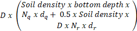
Downward load = D × (Soil density × bottom depth × Nq × dq + 0.5 × Soil density × D × Nr × dr)
= 12.75 × ((120/1728) × 102.375” × 14.39366 × 2.18188 + 0.5 × (120/1728) × 12.75” ×9.37834×2.18188) = 12.75 × 232.3305 lb / in = 106639.7 lb (for 36”) (CAEPIPE: 106640 lb)
Downward stiffness = 25 × 106639.7 / 12.75
= 209097 lb/in (CAEPIPE: 209098)
Vertically Upward Direction
top depth = 96” – 12.75”/2 = 89.625”
Upward load = D × Soil density × top depth
= 12.75” × (120/1728) × 89.625
= 79.35547 lb / in
= 2856.7968 lb (for 36”) (CAEPIPE: 2856.8)
Upward stiffness = 25 × 2856.7968 / 12.75 = 5601.56 lb/in (CAEPIPE: 5601.6)
Verification of cohesive restraints (for pipe element 20 to 30)
Sp = soil pressure = soil density × depth
depth = –1’ – (–5’) = 4’ (since the pipe centerline is at -5’ and ground level is at -1’).
Sp = 150 lbf/ft3 × 4 ft = 600 lb / ft2 = 4.16667 lb/in2
D = 12.75” + (2 x 2.0) = 16.75” (as insulation thickness is defined as 2” and the option “Include Insulation Thickness” is turned ON in Soil S2 input).
Axial direction
Soil strength = Cs = 100 psi = 100 × 6.89476 KN/m2 = 689.476 KN/m2
Af = Adhesion factor = 1.7012775 e(-0.00833699 Cs)[where Cs should be in KN/m2]
= 5.424795E-3
Axial load = p× D × Af × Cs
= p×16.75”×5.424795E-3×100 psi
= 28.54 lb / in
= 1027.66 lb (for 36”) (CAEPIPE: 1027.7)
Axial stiffness = 25 × 1027.66 / 16.75 = 1533.82 lb /in (CAEPIPE: 1533.8 lb/in)
Transverse direction
Transverse load = D × (2 Cs + Sp + 1.5 Cs × depth / D)
= 16.75” × [(2.0×100 + 4.166667 + (1.5×100×48/16.75)]
= 10619.79 lb/in
= 382312.5 lb for 36” (CAEPIPE: 382313)
Transverse stiffness = 25 ×382312.5 / 16.75
= 570615.67 lb /in (CAEPIPE: 570616)
Vertically Downward direction
bottom depth = 48” + 16.75”/2 = 56.375”
= 16.75” × [(5.7182×100) + ((150/1728) × 56.375”)]
= 9659.95 lb/in
= 347758.34 lb for 36” (CAEPIPE: 347758)
Downward stiffness = 25 ×347758.34 / 16.75
= 519042.30 lb / in (CAEPIPE: 519042)
Vertically Upward Direction
top depth = 48” – 16.75”/2 = 39.625”
Upward load = D × Soil density × top depth + 2 Cs × top depth
= 16.75” × (150/1728) × 39.625” + (2×100×39.625”)
= 7982.61 lb / in
= 287374.12 lb for 36” (CAEPIPE: 287374)
Upward stiffness = 25 ×287374.12 / 16.75
= 428916.60 lb / in (CAEPIPE: 428917)
References
1. Tomlinson, M. J., Pile Design and Construction Practice. Fourth Edition. London: E & FN Spon, 1994.
2. Fleming, W.G.K., et al. Piling Engineering. Second Edition. Blackie Academic and Professional. (Chapters 4 and 5).
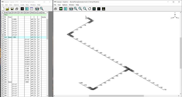
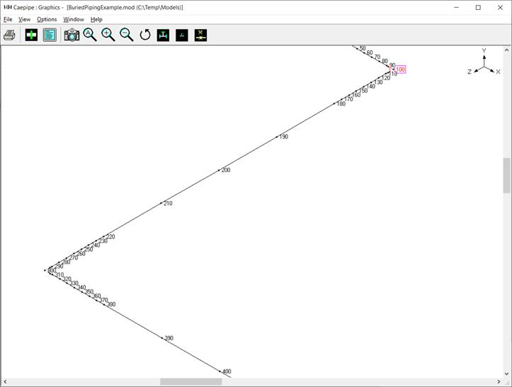
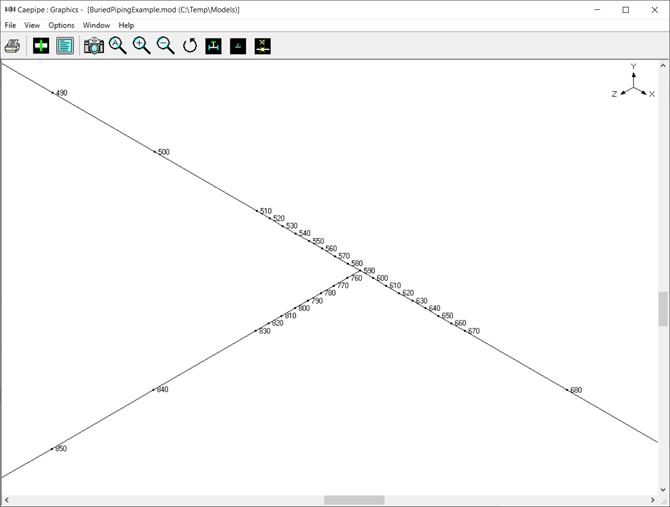
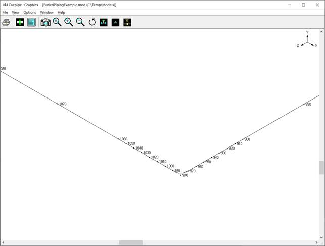
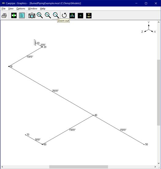
Discretization Example
Soil characteristics
Soil density, w = 130 lbf/ft3 = 0.075 lb/in3
Pipe depth below grade, H = 12 ft (144 in)
Type of backfill, dense sand (cohesionless soil)
Ck = 80
Calculation of Modulus of subgrade reaction (k)
Nh = 0.285H/D + 4.3
Nh = (0.285 x 144 / 12.75) + 4.3 = 7.518
Calculation of Influence Length (Lk)
Moment of inertia, I = 279.3 in4
Modulus of elasticity, E = 27.9 x 10⁶ psi
Pipe / Soil System Characteristics = = [575.127 / (4 x 27.9 x 106 x 279.3)] 1/4 = 0.01165
Influence Length (Lk) = 3 x 3.14 / (4 x 0.01165) = 202.145 in
As the lengths of pipe elements near the bends and branch connection are greater than the influence length (Lk = 202.145 in), the pipe elements near the bends and branch connection are split into a number of short elements with length of each short element being equal to 2 x OD = 2 x 12.75 = 25.5 in until the influence length (Lk). See figures given below for details.