Dynamic Analysis

Modal Analysis

The equations of motion for an undamped lumped mass system may be written as:

(1)

Where

= diagonal mass matrix

= displacement vector

= acceleration vector

= stiffness matrix

= applied dynamic force vector

If the system is vibrating in a normal mode (i.e., free not forced vibration), we may make the substitutions

to obtain

(2)

where

is the vector of modal displacements of the

mode (eigenvector).

Thus we have an eigenvalue (characteristic value) problem, and the roots of equation (2) are the eigenvalues (characteristic numbers), which are equal to the squares of the natural frequencies of the modes.

In CAEPIPE, the eigenvalue problem is solved using a determinant search technique. The solution algorithm combines triangular factorization and vector inverse iteration in an optimum manner to calculate the required eigenvalues and eigenvectors. These are obtained in sequence starting from the lowest eigen-pair [

]. An efficient accelerated secant procedure which operates on the characteristic polynomial

is used to obtain a shift near the next unknown eigenvalue. The eigenvalue separation theorem (Sturm sequence property) is used in this iteration. Each determinant evaluation requires a triangular factorization of the matrix

. Once a shift near the unknown eigenvalue has been obtained, inverse iteration is used to calculate the eigenvector. The eigenvalue is obtained by adding the Rayleigh quotient correction to the shift value. The eigenvector

, has an arbitrary magnitude and represents the characteristic shape of that mode.

Starting from Version 10.40, the determinant of the characteristic polynomial is stored in the power form with an exponent of the order of matrix size. With this improvement in Modal analysis algorithm, CAEPIPE can now extract much higher modes (Eigen vectors) up to the frequency of 9999 Hz.

Orthogonality

For any two roots corresponding to the n^th and m^th modes, we may write equation (2) as which is the orthogonality condition for eigenvectors.

	(3)
	(4)

If we post multiply the transpose of (3) by

, we obtain

or	(5)
Pre multiplying (4) by	(6)

Since

is a diagonal matrix,

. Also, since

is a symmetric matrix,

. The left sides of equations (5) and (6) are therefore equal.

Subtracting (6) from (5),

(7)

Since

(8)

which is the orthogonality condition for eigenvectors.

Modal Equations

Since the eigenvectors (modal displacements) may be given any amplitude, it is convenient to replace

such that

(9)

The eigenvectors are evaluated so as to satisfy equation (9) and at the same time keep the displacements in the same proportion as those in

. The eigenvectors are then said to be normalized. Note that equation (7) is still satisfied since, if n = m,

, and the remaining terms may be given any desired value.

Equation (2) now may be written for the n^th mode as

Let

be a square matrix containing all normalized eigenvectors such that the n^th column is the normalized eigenvector for the n^th mode. We can therefore write the matrix equation so as to include all modes as follows:

(10)

Where

is a diagonal matrix of eigenvalues. We now premultiply both sides of (10) by

to obtain

(11)

It may be shown that

(12)

where [

] is the unit diagonal matrix. Equation (12) can easily be verified by expansion and follows from the orthogonality condition and the fact that

has been normalized. Equation (11) therefore can be written as

(13)

Returning now to the equation of motion (1),

let

and

(14)

Where

is the modal amplitude of the n^th mode. This merely states that the true modal displacements equal the characteristic displacements (eigenvector displacements) times the modal amplitude determined by the response calculations and, further that the total displacements are linear combinations of the modal values. If we now pre-multiply equation (1) by

and substitute equations (14), we obtain

(15)

Substituting from equations (12) and (13) in equation (15),

(16)

which represents the modal equations of motion.

Uniform Support Motion

Solutions for uniform support motion (when all supports experience the same excitation) may be obtained if

is replaced by

where

is the prescribed support acceleration. Thus, the modal equations of motion may be written as

(17)

where

is the relative modal displacement for the n^th mode with respect to the support.

The participation factors for the modes is given by

(18)

Then the modal amplitude contribution from the n^th mode is given by

(19)

Where

is the response of a single degree of freedom system having circular frequency

. Using equations (14) and (19), the total displacements from M modes are given by

(20)

Effective Modal Mass

Effective modal mass is defined as the part of the total mass responding to the dynamic loading in each mode. When the participation factor is calculated using normalized eigenvectors as in equation (18), the effective modal mass for the n^th mode is simply the square of the normalized participation factor,

(21)

Effective modal mass is useful to verify if all the significant modes of vibration are included in the dynamic analysis by comparing the total effective modal mass with the total actual mass.

Independent Support Motion (Multi-level Response Spectrum Analysis)

When the piping is routed along the wall of a tall building, the piping supports at higher elevation floors of the building will experience higher seismic excitations, whereas the piping supports at the ground level will experience lesser seismic excitation. Likewise, a pipeline crossing over a bridge may experience different seismic excitations at the ends. Piping systems with such multiple seismic excitations can be analyzed in CAEPIPE using Multi-level Response Spectrum Analysis. For any number of levels in a system, the participation factor for the n^th mode with k^th level excitation is given by

(22)

where,

is the influence vector representing the simultaneous displacements of all the supports located at k^th level.

Then the modal amplitude contribution from the n^th mode is given by

(23)

where, L is the number of levels and

is the response of a single degree of freedom system having a circular frequency

. The total displacements are given by

(24)

Notes:

1) Two (2) types of combinations “SRSS” and “ABS” can be performed for Level Summations in CAEPIPE The combination over level contributions will be performed first, followed by interspatial and then intermodal combination without the consideration of closely spaced modes. This is consistent with present NRC guidelines.

2) For Multi-level Response Spectrum Analysis, Missing mass correction is available in CAEPIPE starting version 11.00. It is still recommended to include a sufficient number of modes in the analysis and ensure that the “Modal mass / Total mass” is sufficiently high (thereby confirming that most of the mass of the system participates in the modes computed) in Global X, Y and Z directions through Results Window > Results > Results… > Frequencies.

References:

Bezler, P., Subudhi, M., & Hartzman, M. (1985). Piping benchmark problems: dynamic analysis independent support motion response spectrum method (NUREG/CR--1677-Vol2). United States

Nakamura, Y., Kiureghian, A.D., & Liu, D. (1993). Multiple-Support Response Spectrum analysis of the golden gate bridge.

Lin, C.W., & Loceff, F. (1980). A new approach to compute system response with multiple support response spectra input. Nuclear Engineering and Design, 60(3), 347-352.

Response Spectrum

The concept of response spectrum, in recent years has gained wide acceptance in structural dynamics analysis, particularly in seismic design. Stated briefly, the response spectrum is a plot of the maximum response (maximum displacement, velocity, acceleration or any other quantity of interest), to a specified loading for all possible single degree-of-freedom systems. The abscissa of the spectrum is the natural frequency (or period) of the system, and the ordinate, the maximum response.

In general, response spectra are prepared by calculating the response to a specified excitation of single degree-of-freedom systems with various amounts of damping. Numerical integration with short time steps is used to calculate the response of the system. The step-by-step process is continued until the total earthquake record is completed and becomes the response of the system to that excitation. Changing the parameters of the system to change the natural frequency, the process is repeated and a new maximum response is recorded. This process is repeated until all frequencies of interest have been covered and the results plotted. CAEPIPE provides fourteen (14) response spectra for your convenience. Refer to Appendix B titled “Response Spectrum Libraries” in CAEPIPE User’s Manual for details.

Since the response spectra give only maximum response, only the maximum values for each mode are calculated and then superimposed (modal combination) to give total response. A conservative upper bound for the total response may be obtained by adding the absolute values of the maximum modal components (absolute sum). However, this is excessively conservative and a more probable value of the maximum response is the square root of the sum of squares (SRSS) of the modal maxima.

To calculate response of the piping system, for each natural frequency of the piping system, the input spectrum is interpolated (linearly or logarithmically). The interpolated spectrum values are then combined for the X, Y and Z directions (direction sum) either as absolute sum or SRSS sum to give the maximum response of a single degree-of-freedom system:

at that frequency.

From equation (20) or (24) the maximum displacement vector for the n^th mode can be calculated from the maximum response

of a single degree-of-freedom system.

The maximum values of element and support load forces per mode are calculated from the maximum displacements calculated per mode as above using the stiffness properties of the structure.

The total response (displacements and forces) is calculated by superimposing the modal responses according to the specified mode sum method which can be absolute sum, square root of sum of squares (SRSS) or closely spaced (10%) modes method.

Closely Spaced Modes

Studies have shown that SRSS procedure for combining modes can significantly underestimate the true response in certain cases in which some of the natural frequencies of a structural system are closely spaced. The ten percent method is one of NRC approved methods (Based on NRC Guide 1.92) for addressing this problem.

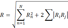
where

= Total (combined) response

= Peak value of the response due to the n^th mode

= Number of significant modes

The second summation is to be done on all i and j modes whose frequencies are closely spaced to each other. Let

and

be the frequencies of the i^th and j^th modes. The modes are closely spaced if:

Time History

Time history analysis requires the solution to the equations

(25)

where

= diagonal mass matrix

= damping matrix

= stiffness matrix

= displacement vector

= velocity vector

= acceleration vector

= applied dynamic force vector

The time history analysis is carried out using mode superposition method. It is assumed that the structural response can be described adequately by the p lowest vibration modes out of the total possible n vibration modes and p < n. Using the transformation

, where the columns in

are the p mass normalized eigenvectors, equation (25) can be written as

(26)

where

= diag

In equation (26), it is assumed that the damping matrix

satisfies the modal orthogonalitycondition

Equation (26) therefore represents p uncoupled second order differential equations. These are solved using the Wilson

method, which is an unconditionally stable step-by-step integration scheme. The same time step is used in the integration of all equations to simplify the calculations.

Random Vibration Analysis for Uniform Base Excitation

A Random Vibration Analysis in CAEPIPE can be used when a structure is subjected to a non-deterministic, continuous uniform base excitation. The solution can be formulated in the frequency domain when the excitations are expressed by power spectral density (PSD) functions. For excitation PSD matrix

, the modal force PSD matrix is defined as

The PSD of modal displacement response is obtained as

Note: At present in CAEPIPE, the Random Vibration Analysis is available for single input (or zero cross mode response) with uniform base excitation.

A zero-delay autocorrelation response becomes.

The mean square response is determined from

Various modal combinations are available: the SRSS Method, Absolute method, CSM, and NRL. The variances for stresses, nodal forces, or reactions are computed from equations similar to those above, where replace the mode shapes with mode stresses, if stress variance is desired. Similarly, if nodal force variance is desired, replace the mode shapes with mode nodal forces. Finally, if reaction variances are desired, replace the mode shapes with mode reactions. The cross-mode response is neglected; that is, the effect of one mode on another is disregarded.

Normal Mode Method: The normal mode method available in CAEPIPE is an efficient method to calculate the response of the system when the large system tends to respond globally only in the first few modes, primarily the fundamental mode. The modes considered to evaluate response are up to the cutoff frequency or the maximum frequency at which PSD Data load is defined, whichever is smaller. In the approximate normal mode method, the PSD of excitations is considered uniform around each natural mode (typically white noise). Ideally, this method will be suitable for white noise exposure or assuming it as white noise PSD load around each natural mode. For approximate method, the mean square responses are determined analytically for the modal responses:

Note 1: At present, the Random Vibration analysis is available for NONE code only where Von Mises stresses are calculated. Refer to the section NONE code in CAEPIPE Code Compliance Manual for details on Von Mises Stress evaluation.

Note 2: At present in CAEPIPE, the Random Vibration Analysis is available for single input (or zero cross mode response) with uniform base excitation.

Note 3: In Random Vibration Analysis, the variance/response of the system is evaluated in the frequency range specified in the PSD Data table. The lowest and highest frequencies specified in the table are the lower and upper bounds of integration. The natural modes falling outside the frequency range of PSD data table will not be considered in the analysis. It is users’ responsibility to specify PSD data across the desired range of frequency.

Fatigue evaluation due to Random Vibration Load

Fatigue evaluation due to Random Vibration excitation (PSD Load) is available in CAEPIPE based on Palmgren-Miner hypothesis, which asserts that fatigue damage is cumulative, and proportional to the applied levels of stress.

It is assumed that the system is exposed to PSD load at 68.3% at 1 Sigma, 27.1% at 2 Sigma and 4.3% at 3 Sigma, where Sigma is variance or standard deviation of Gaussian distribution and “n” is the total number of applied cycles. The failure occurs when cumulative load cycling exceeds 1 i.e.,

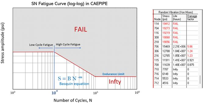
Failure criteria for Random Vibration fatigue: SN Fatigue Curve

CAEPIPE employs SN Curve Equation (Basquin Equation) as a failure criterion. Refer to Materials section of CAEPIPE Technical Reference Manual for the input parameters of the Basquin equation and Endurance Limit.

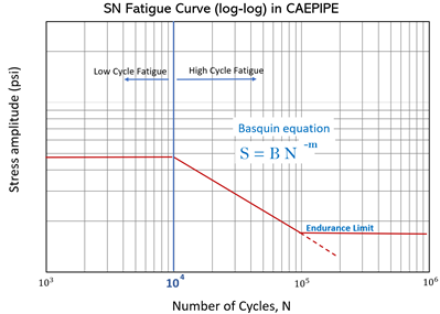
CAEPIPE utilizes the Basquin equation to assess high cycle fatigue, applicable when the number of cycles exceeds 10,000 and maximum up to its endurance limit, as shown in the above figure. It is assumed that for any given material of the pipe, it can endure infinite cycles of load below endurance limit of stress. For low cycle fatigue, a constant allowable stress limit is assumed for simplification, where the Basquin curve intersects the 10,000-cycle mark.

In summary, for any single occurrence of stress above the red line (i.e. grey zone in below figure), the CAEPIPE will show a result of “FAIL” in the sorted stress table. Conversely, if all instances of 1 Sigma, 2 Sigma, and 3 Sigma stresses remain beneath the endurance stress limit, then CAEPIPE will indicate “Infty” (meaning infinite life). Otherwise, the software calculates life expectancy (in hours) based on the Steinberg Theory. If the user provides exposure time, CAEPIPE will also calculate the damage factor for the specified duration of piping exposure to random vibration.

Reference:

Matjaz Mrsnik, Janko Slavic and Miha Boltezar, Frequency-domain methods for a vibration-fatigue-life estimation - Application to real data. International Journal of Fatigue, Vol. 47, p. 8-17, 2013. DOI: 10.1016/j.ijfatigue.2012.07.005