Force Spectrum

Force spectrum analyses (different from harmonic analyses) are generally performed to determine the response of the piping system to short-duration impulsive loads such as fluid hammer, safety relief valve (SRV) and slug flow loads. For an actual short-duration impulsive dynamic load exerted on a piping system, a fluid transient analysis is first carried out in order to arrive at the “time-history loads” (i.e., force vs. time) acting in the three global directions (namely global X, Y and Z) at all affected points in the piping system. The time-history load sets so computed are then applied, one time-history load set at a time, on a single degree-of-freedom spring-mass system with a pre-set natural frequency, to determine the maximum dynamic response of this single degree-of-freedom system with that natural frequency. Such dynamic analysis for that time-history load is repeated on the same single degree-of-freedom system with different pre-set natural frequencies. The force spectrum for that time-history load would then be a table of maximum dynamic response computed for the single degree-of-freedom system with different natural frequencies. In other words, the force spectrum is a table of force spectral values vs frequencies that captures the maximum intensity and frequency content of that time-history load. Similarly, force spectrum tables are determined for all other time-history load sets. The above force spectrum tables (i.e., maximum dynamic force vs frequency) are then applied as inputs at the respective piping nodes of the CAEPIPE stress model to compute displacements, forces and stresses.

For any piping system, there are as many natural modes of vibrations as the number of dynamic degrees of freedom for that system. The force spectral value corresponding to a natural frequency of the piping system is arrived at by interpolating the force spectrum vs frequency table as determined above. For better understanding, as an example, refer to the graph shown next as well as the natural frequencies computed for a piping system at 10 Hz, 14 Hz, 21 Hz, 29 Hz and 33.8 Hz.

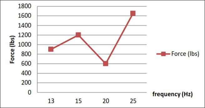
From the above graph, to arrive at a force value corresponding to a natural frequency of 14 Hz, CAEPIPE interpolates the force spectral values between 13 and 15 Hz. Similarly, to arrive at a force value corresponding to a natural frequency of 21 Hz, CAEPIPE interpolates the force spectral values between 20 Hz & 25 Hz. Since force spectral values above 25 Hz are not defined in the graph shown above, CAEPIPE arrives at a force value of 1650 lb. (i.e., the spectral value corresponding to the maximum frequency of 25 Hz in the above plot) even for natural frequencies of 29 and 33.8 Hz. Similarly, CAEPIPE arrives at a force value of 900 lb. for a natural frequency of 10 Hz (i.e., the spectral value corresponding to the minimum frequency of 13 Hz in the above plot).

If only one set of force versus frequency is input (for example, 1000 lb. at 14 Hz) in the force spectrum table for your model, CAEPIPE applies the same force (1000 lb.) for all natural frequencies computed for that piping system. Note that the displacement produced at a node will remain unchanged even when the sole frequency in the force spectrum table is changed from 14 Hz to any other frequency.

Here, the results of the modal analysis are used with force spectrum loads to calculate the response (displacements, support loads and stresses) of the piping system. It is often used in place of a time-history analysis to determine the response of the piping system to sudden impulsive loads such as water hammer, relief valve and slug flow. The force spectrum is a table of spectral values versus frequencies that captures the intensity and frequency content of the time-history loads. It is a table of Dynamic Load Factors (DLF) versus natural frequencies. DLF is the ratio of the maximum dynamic displacement divided by the maximum static displacement. Note that Force spectrum is a non-dimensional function (since it is a ratio) defining a curve representing force versus frequency. The actual force spectrum load at a node is defined using this force spectrum in addition to the direction (FX, FY, FZ, MX, MY, MZ), units (lb, N, kg, ft-lb, in-lb, Nm, kg-m) and a scale factor.

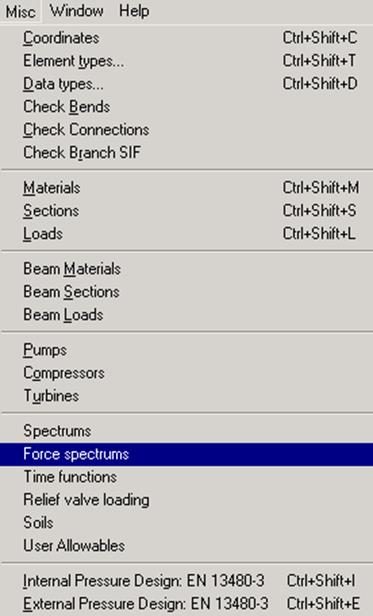
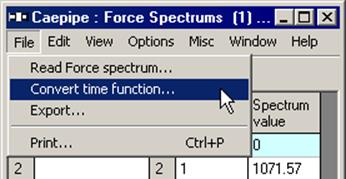
The Force spectrums are input from the Layout or List menu: Misc > Force spectrums.

The Force spectrum list appears.

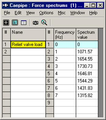
Enter a name for the force spectrum and spectrum values versus frequencies table. In addition to inputting the force spectrum directly, it can also be read from a text file or converted from a previously defined time function.

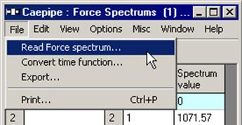
To read a force spectrum from a text file:

use the List menu: File > Read force spectrum.

The text file should be in the following format:

Name (up to 31 characters)

Frequency (Hz) Spectrum value

. .

The frequencies can be in any order. They will be sorted in ascending order after reading from the file.

To convert a previously defined time function to force spectrum:

use the List menu: File > Convert time function.

The Convert Time Function dialog appears.

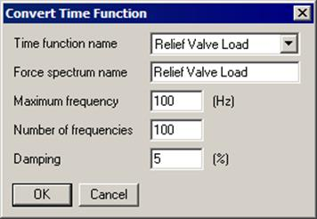
Select the time function to convert from the Time function name drop down combo box. Then input the Force spectrum name (defaults to the Time function name), Maximum frequency, Number of frequencies and the Damping. When you press Enter or click on OK, the time function will be converted to a force spectrum and entered into the force spectrum list.

The time function is converted to a force spectrum by solving the dynamic equation of motion for a damped single spring mass system with the time function as a forcing function at each frequency using Duhamel’s integral and dividing the absolute maximum dynamic displacement by the static displacement.

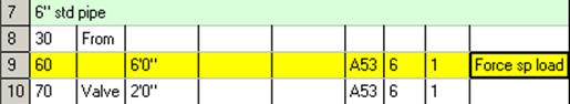
Force Spectrum Load

The force spectrum loads are applied at nodes (in Data column in Layout window). At least one force spectrum must be defined before a force spectrum load at a node can be input.

To apply the force spectrum load at a node click on the Data heading or press Ctrl+Shift+D for Data Types dialog.

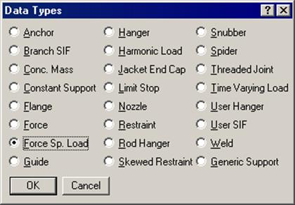
Select “Force Sp. Load” as the data type and click on OK. This opens the Force Spectrum Load dialog.

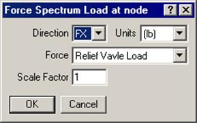
Select the direction, units and force spectrum using the drop down combo boxes and input appropriate scale factor. The scale factor can be a scalar value, which, when multiplied by the non-dimensional force spectrum, will give the actual magnitudes of the force versus frequency in the global direction and unit selected in the above dialog. Then click on OK to enter the force spectrum load at that node.

Input force spectrum loads at other nodes similarly. Then select the force spectrum load case for analysis using the Layout menu: Loads > Load cases.

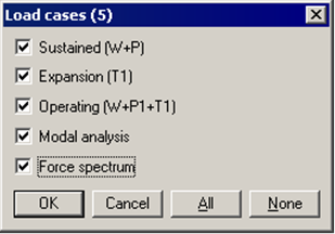
Note that Modal analysis and Sustained (W+P) load cases are automatically selected when you select Force spectrum load case. The force spectrum load case is analyzed as an Occasional load.

A Relief Valve Analysis may be performed by first obtaining the data about valve opening and subsequent behavior, as a force versus time history profile. Enter the profile as a time function. See under Time History Load for how to.

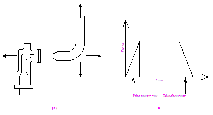
Then under Force Spectrum, use “Convert time function” to convert the force-time history profile into a Force-Spectrum. Input loads and analyze. See the topic Relief Valve Load Analysis for more details.