Time functions
Time functions are non-dimensional tables (i.e., a series of time versus value pairs) which describe the variation of the forcing function with time. Usually, a transient fluid flow analysis program computes forces as a function of time at all changes in directions (bends/tees) and other points of interest. These forces/moments result from a transient event such as a fluid hammer. Separate force-time histories are then input as time functions and applied as Time Varying Loads within CAEPIPE at the Data column of the corresponding nodes of interest in the piping model.
In CAEPIPE, the time function you define can have any interval between two time values. You can make that table as fine as you want it to be.
You must have a zero entry for the Value next to the first Time input. Time history analysis begins at time t=0.0. You can input as many time-value pairs as required.
There are two methods for inputting time functions.
1. Input time functions directly into the model.
2. Create a text file for each function and read it into CAEPIPE.
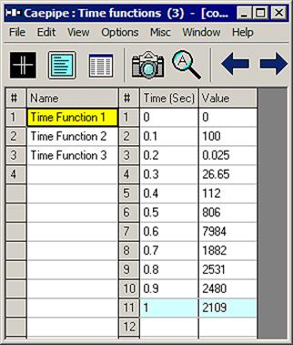
Click on menu Misc > Time functions to type in time functions. Time is measured in seconds. Value is non-dimensional. You can assign units to these Values when you input a Time varying load at a node. For now, simply start typing the time-value pairs. Next, input parameters for the Time History Analysis Control dialog, and then input Time Varying Loads at nodes of interest.
2. Create a text file for each function and read it into CAEPIPE
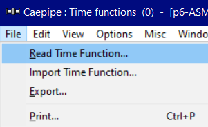
Read text files into CAEPIPE using the menu File > Read Time Function command. For each function, you need to type a Name (up to 31 characters) on the first line, type time followed by a Value (separated by a space) on the following line. You can input as many time-value pairs (one pair on each line) as required. If you have more than one time functions then they can be defined in the same file by adding the tag “-1.e11” at the end of each time function. Flow master exports the Time functions in the format given below.
The format of the time function text file is shown below. The time function that is read from a file appears on the row where the yellow highlight is placed (under the Name column). You can use the Edit menu commands to insert an empty row or delete an existing time function. Ensure that no two time functions share the same Name. CAEPIPE issues a warning should such occur.
Time Function 1
0.0 0
0.1 0
0.2 0.025
0.3 26.65
0.4 112
0.5 806
0.6 7984
0.7 1882
0.8 2531
0.9 2480
1 2109
. .
. .
-1.e11
Time Function 2
0
0.1 0.035
0.2 28.000
0.3 120
. .
. .
3. Import time functions from AFT Impulse / PIPENET software into CAEPIPE
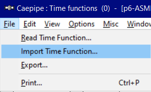
Import AFT Impulse /PIPENET force difference file into CAEPIPE using the menu File > Import Time Function command.
Given below is a snapshot of frc file from AFT Impulse.
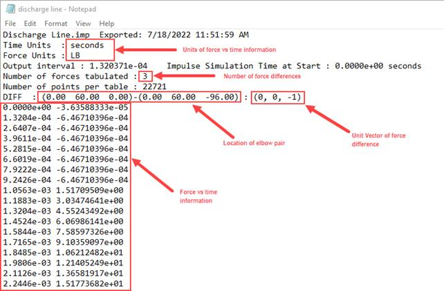
CAEPIPE will assign the name of the Time function as equal to the system tag given in the first line (up to 26 characters or the characters until the tag “.imp”) of the AFT Impulse frc file with suffix “-FXXXX” added, where XXXX is the running number from 1 through 9999”. On the other hand, CAEPIPE will assign the name of the Time function as equal to tag name stated in the line DIFF for PIPENET frc file.
For example, when the sample frc file shown above from AFT Impulse is imported into CAEPIPE, it will assign the name of the first time function as “Discharge Line-F1”.
Lines 2 through 6 will be ignored from AFT file as they are NOT required in the Time Function values input in CAEPIPE. Each Time function is identified by CAEPIPE using the tag “DIFF” available in the AFT Impulse frc file.
Given below is a snapshot of frc file from PIPENET.
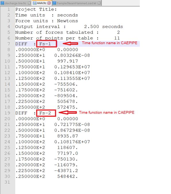
When a frc file shown from PIPENET is imported into CAEPIPE, it will assign the name of the Time function as the value stated after “:” in the line starting with “DIFF”.
For example, when the sample frc file shown above from PIPENET is imported into CAEPIPE, it will assign the first and second Time function name as “Fs-1” and “Fs-2” respectively.
Lines 1 through 6 will be ignored from PIPENET file as they are NOT required in the Time Function values input in CAEPIPE. Each Time function is identified by CAEPIPE using the tag “DIFF” available in the AFT Impulse frc file.
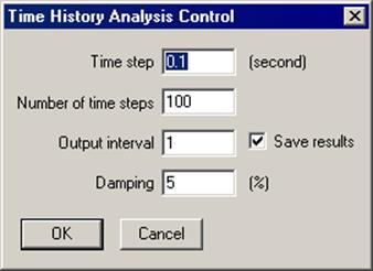
Once you are done entering or importing time functions, specify the parameters in the Time History Analysis Control dialog under menu Loads > Time History, details of which are provided earlier under the Loads menu topic.
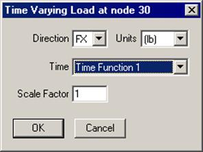
Then, specify Time Varying Loads at applicable nodes in the model. The following figure shows the time function as a time-varying force applied in the X direction (FX) at node 30. Under Units, you can specify one of several depending on whether you are applying the Values in the time function as a force (FX, FY, FZ) or a moment (MX, MY, MZ). For more details, please see discussion under menu Loads > Time History.