Tutorial for Modeling Victaulic Coupling in CAEPIPE
The following are the Steps for modeling and including Victaulic Coupling in CAEPIPE analysis.
General
Victaulic is a developer and producer of mechanical pipe joining systems and is the originator of the grooved coupling pipe joining system.
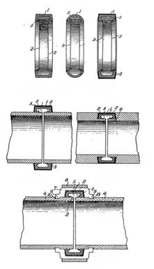
Victaulic Grooved Couplings are used to join mechanical pipes together. Grooved coupling pipe joining systems use a roll grooving technique to join pipes and pipe joining components. A groove is placed at the end of two pipes to prepare the pipes engagement with the coupling housing and gasket. The gasket creates a pressure responsive seal on the outside diameter of the pipe, unlike standard compression joints, where pressure acts to separate the seal. The gasket sealing is enhanced as the coupling housing is tightened onto the pipe end. "The economics of the grooved method derive from simplified assembly that involves three basic concepts: a pressure responsive gasket that creates a leak-tight seal; couplings that hold the pipes together; and fasteners that secure the couplings.
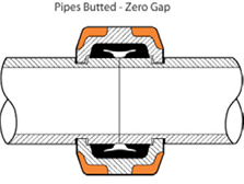
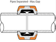
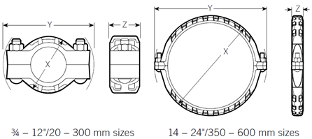
Mechanical piping joining systems are being used in HVAC, plumbing, fire protection and mining, water and waste water treatment, oilfield operations, power plants, military, marine systems and other industrial applications due to the time and labor-saving features associated with installation. Mechanical piping joining systems offer an alternative to welding, threading, and flanging for joining two pipe ends. See the figures given below for details.
The steps provided in this tutorial are applicable for most of the Victaulic Couplings, including Styles 77 and 177. The properties for Style 77 are referred from the document available in the link http://static.victaulic.com/assets/uploads/literature/06.04.pdf. Dimensional details and mechanical properties of Victaulic Coupling are referred from the document given in the above link corresponding to 12” Victaulic Coupling. The same is presented below for quick reference.
The following report gives a tutorial on modelling Rigid and Flexible Victaulic Couplings in CAEPIPE.
Part 1 - Tutorial for Modeling Rigid Victaulic Coupling
Rigid Victaulic Coupling Catalogue
The Manufacturer’s Catalogue for Rigid Victaulic Coupling is shown below for your quick reference.
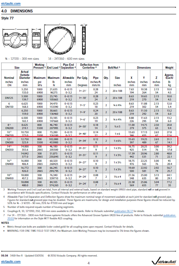
The .pdf file of the details of Style 77 Victaulic Couplings downloaded from the link mentioned above is attached herewith for convenience.
Rigid Victaulic Grooved Couplings provide a permanent pipe connection which can withstand full pressure thrust loads at their maximum rated working pressure. Victaulic rigid couplings positively clamp the pipe to create a rigid joint, so axial movement and angular deflection are eliminated. They are particularly useful on risers, mechanical rooms, horizontal runs with numerous branches and other areas where flexibility is not required. Proper rigid coupling installation provides system behavior characteristics similar to those of other rigid systems, in that all piping remains strictly aligned and is not subject to axial or angular movement during operation. For this reason, systems installed with Victaulic rigid couplings utilize support techniques identical to those used in welded systems. This Rigid Victaulic Coupling can be best represented in CAEPIPE using an element called “Ball joint” with its Rotational and Torsional stiffnesses as ‘Rigid’ and its Rotational and Torsional limits as NONE.
Step 1:
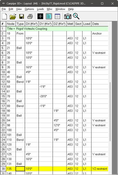
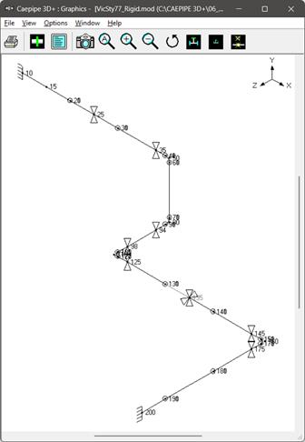
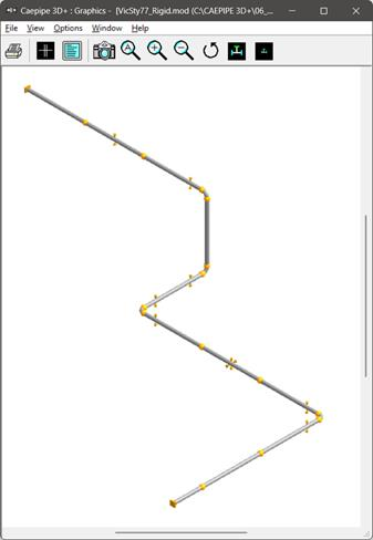
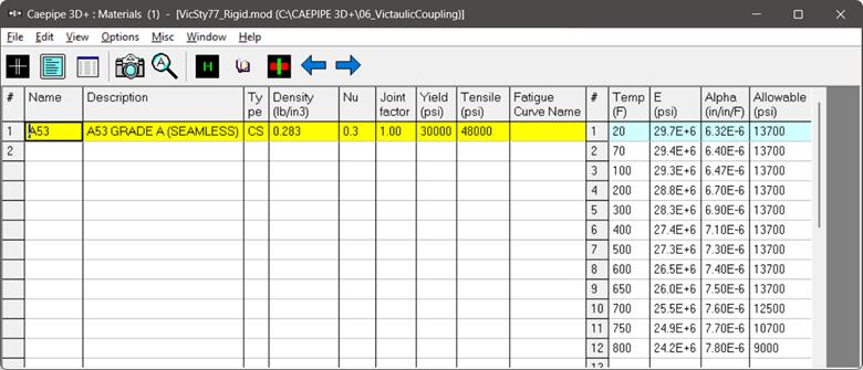
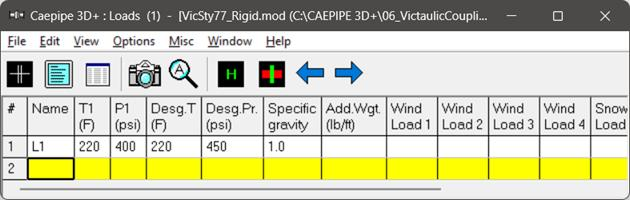
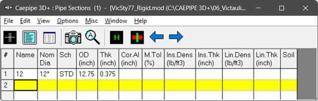
Attached is a sample CAEPIPE Stress layout with Rigid Victaulic Couplings (see the “vicsty77_rigid.mod” file). Snapshots of the piping layout along with its details are shown below.
Step 2:
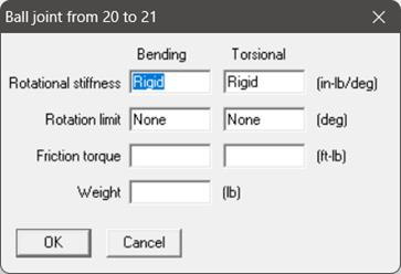
You may observe that all of the Victaulic Couplings are modeled using “Ball joints” in CAEPIPE. As an example, the dialogue box corresponding to the Victaulic Coupling (Ball joint) between nodes 20 and 21 is shown below.
Step 3:
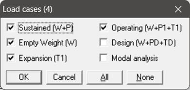
Select the required Load Cases through ‘Layout Window > Loads > Load cases’. Save the model and perform the analysis through ‘Layout window > File > Analyze’.
Step 4:
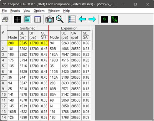
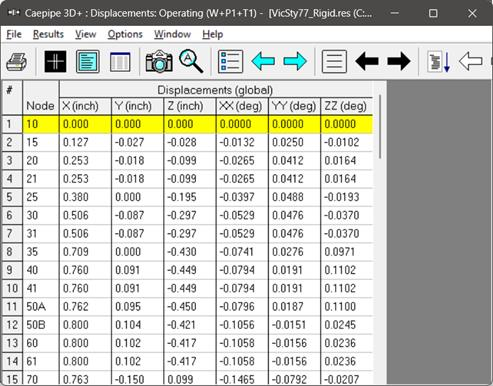
The sorted stress, displacements, and support loads of the results are shown below.
Step 5:
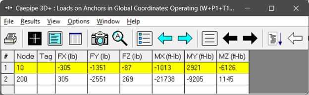
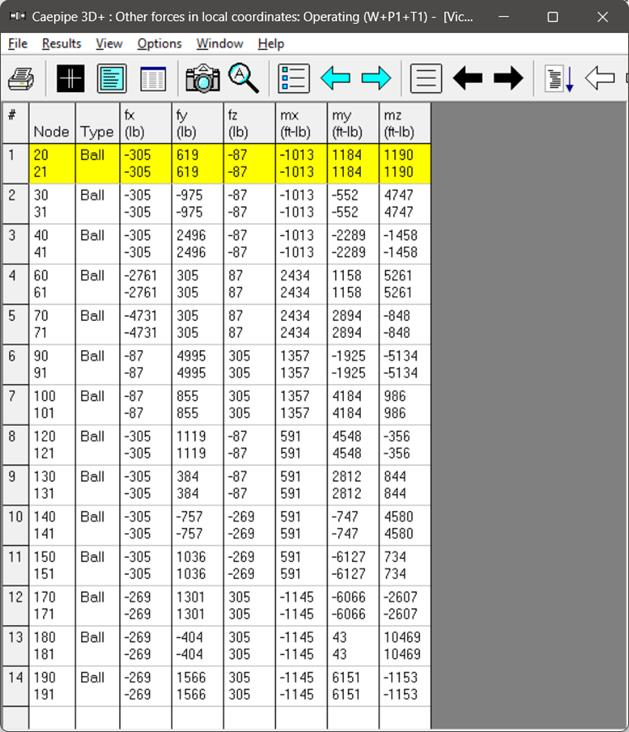
Loads computed at the Ball joints (Victaulic Couplings) can be seen through “Results Window> Results > Element forces” and then, “Results Menu > Results > Other forces > Other”. The forces shown below for operating load case 1 (W+P1+T1) results can then be compared against the ‘End Loads’ provided in the Victaulic Coupling Manufacturer’s Catalogue (shown above).
For example, for the considered 12” Victaulic Couplings in the model, the ‘End Load’ provided in the Victaulic Coupling catalogue is 102,000 lbs which is greater than the maximum of all the Ball joint forces (fx, fy & fz).
Summary
From the above exercise, it is noted that the loads (fx, fy &fz) at all Victaulic coupling locations (ball joints) computed by CAEPIPE for Operating Load Case 1 are less than the respective Maximum Permissible End Load (102000 lb) provided in the Catalog thereby meeting the criteria.
Part 2 - Tutorial for Modeling Flexible Victaulic Coupling
Flexible Victaulic Couplings permit controlled pipe movement within the couplings while they maintain a positive seal and self-restrained joint. This is achieved because the coupling key section engages but "floats" in the groove. The design allows for expansion, contraction and angular deflection generated by thermal changes, building or ground settlement, and seismic activity. Pipe movement accommodation by Victaulic flexible couplings will minimize the stresses that can be generated by this movement. Victaulic flexible couplings also have superior vibration attenuation characteristics.

This Flexible Victaulic Coupling can be simulated in CAEPIPE using “Bellow and a Tie Rod” as shown in part 2 of this tutorial titled “Tutorial for Modelling Rigid Victaulic Coupling”. Flexible Victaulic Coupling Stiffnesses can be obtained from the manufacturer or else, they can be hand calculated using the dimensional properties provided in the Victaulic Coupling Catalogue as shown in the sample calculations provided below.
Axial, lateral, and torsional Stiffnesses of Victaulic AGS Flexible Coupling, Style W77 are not available in the manufacturer’s catalog. Hence, these values are calculated manually using the dimensions X, Z, and outer diameter of pipe (=ID of coupling) provided in the Victaulic Coupling Catalogue given above and entered in the stress model.
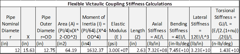
The properties of NS 12” Victaulic Coupling thus computed are shown below.
Flexible Victaulic Coupling Stiffness Calculation
Step 1:
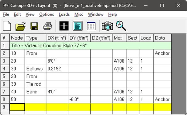
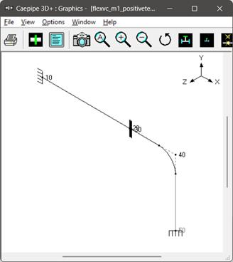
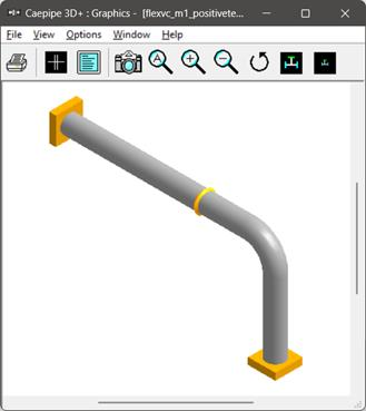
Shown below is a sample CAEPIPE model with Flexible Victaulic Coupling (see the “flexvc_m1_positivetemp.mod” file). As stated above, Flexible Victaulic Coupling is modeled using a combination of Bellow and a Tie Rod between nodes 20 and 30.
Step 2:
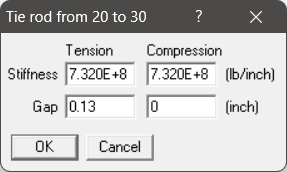
Axial Stiffness of the Tie Rod in Compression and Tension = AE/L = 7.32E+8 lb/inch (as shown in the table above)
Gap in Tension = 0.13” (= Maximum Separation for Roll Groove – Minimum Separation for Roll Groove = 0.13” – 0.0”)
Gap in Compression = 0” (as the coupler cannot compress any further beyond Minimum Separation)
The above parameters are entered for Tie Rod between Node 20 and 30, as shown in the snapshot below.
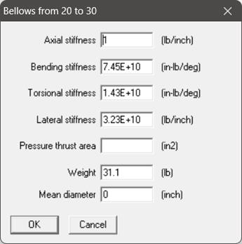
Lateral, bending and torsional stiffnesses of the flexible Victaulic Coupling are entered in Bellow’s Input Dialogue as shown below. Since the axial stiffness fo the flexible Victaluic Coupling is already input in Tie Rod, the same is entered as 1 (Very Small Non-Zero Number) in Bellow’s dialogue.
Step 3:
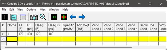
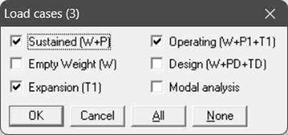
Select the Load Cases shown below for analysis through Layout Window > Loads > Load cases. Save the model and perform the analysis through Layout window > File > Analyze.
Step 4:
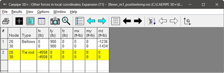
From the Displacements and Element forces results of CAEPIPE for “Operating (W+P1+T1)” Load case for the model with temperature Increase, note the following.
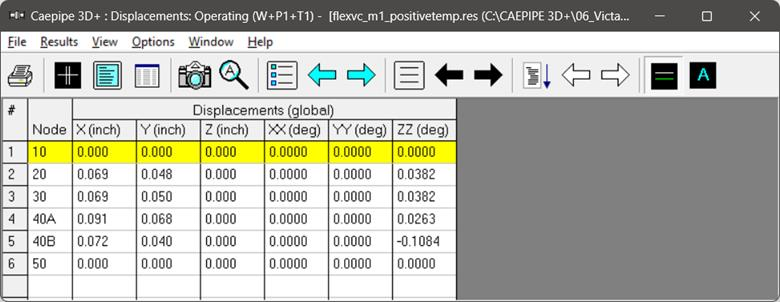
The differential Axial displacement between Nodes 20 and 30 = abs[0.069 – (0.069)] = 0.0” < 0.13” (Pipe End Separation specified in the catalog 0.13”).
The differential Angular Deflection = abs[0.0382 – 0.0382)] = 0 deg < 0.58 deg (Allowable Deflection specified in the catalog).
Axial Load at Tie Rod = -4598 lb < 102000 lb (End Load specified in the catalog).
Summary
From the above exercise, it is noted that the differential Axial displacement, differential Angular rotation and Axial load at Tie Rod computed by CAEPIPE for Operating Load Case 1 for Coupling modeled between Nodes 20 and 30 for Temperature Increase are less than the respective Allowable Linear Movement (0.13”), Angular Deflection (0.58 deg) and Maximum Permissible End Load (102000 lb) provided in the Catalog, thereby meeting the criteria.