Tutorial for Response Spectrum Analysis using CAEPIPE

General

· The Response Spectrum is a plot of the maximum response (maximum displacement, velocity, acceleration or any other quantity of interest) to a specified dynamic loading applied on all possible single degree-of-freedom systems. The abscissa of the spectrum is the natural frequency (or period) of the system, and the ordinate is the maximum response.

In general, response spectra for a seismic event are prepared by calculating the maximum response to a specified ground motion excitation of single degree-of-freedom systems with various amounts of damping. Numerical integration with short time steps is used to calculate the response of each single degree-of-freedom system. The step-by-step process is continued until the total earthquake record is completed, the results of which becomes the response of that system to that excitation. Change the parameters of the system to change its natural frequency, repeat the process for the same excitation and record the new maximum response. This process is repeated until all frequencies of interest have been covered and the results plotted. Typically the El Centro, California earthquake of 1940 is used for this purpose. Attached (“ElCentro.txt”) is an ASCII file that contains spectrum from El Centro, California earthquake of 1940. [First line in this file is the name of the spectrum. Second line defines the “Units” for Abscissa (X-axis) and Ordinate (Y-axis) axes, separated by a space. Starting from the 3^rd line, the first column is Abscissa and the second column is Ordinate. For further details on this ASCII file, refer to the “Spectrums” subsection under “Misc.” section of Menus in the CAEPIPE User’s Manual.]

· Response Spectrum thus prepared as explained above is then input/imported into CAEPIPE Stress model for analysis through CAEPIPE Layout window > Misc > Spectrums.

· Once the inputting of different spectrums are done, input the Spectrum levels applicable for the current analysis through Layout window > Loads > Spectrum. Define a single level for uniform response spectrum analysis. For piping supported at different elevations with each elevation experiencing different seismic loads, define multiple levels with the corresponding spectrum loads. In the latter case, the levels should be assigned to each support.

· Save the model and perform analysis using CAEPIPE.

· Spectrum load specified will be applied at all supports, following which CAEPIPE will compute the modal and directional responses, which are further combined as per the combination method selected.

· Since the response spectra give only maximum response, only the maximum values for each mode are calculated and then superimposed (modal combination) to give a total response. A conservative upper bound for the total response may be obtained by adding the absolute values of the maximum modal components (absolute sum). However, this is excessively conservative and a more probable value of the maximum response is the square root of the sum of squares (SRSS) of the modal maxima.

· Ensure the CAEPIPE results meet project specific analysis requirements. If not, make changes to the piping layout and/or changes to support types and their locations and then reanalyze the model until the analysis requirements are met.

Uniform Response Spectrum Analysis

The following are the Steps for performing the Uniform Response Spectrum Analysis using CAEPIPE.

Step 1:

Attached is a sample CAEPIPE model with Response Spectrum. The piping layout shown below (extracted from the attached model) is for a water supply line that has the following layout and properties. The Analysis Code is selected as ASME B31.9 for this sample model.

Step 2:

Input Spectrums into CAEPIPE. This can be done in three ways:

Input spectrums directly into the model.

Create a spectrum library and load spectrums from it.

Input spectrums from a text file.

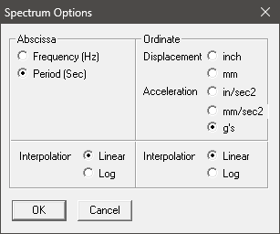
When the first two methods are used, the units for the X-axis and Y-axis as well as the interpolation method are set through the menu Options > Spectrum.

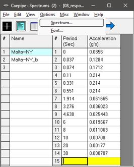
For the sample layout described above, spectrum was input directly into CAEPIPE model manually. If you wish to read the spectrum file “ElCentro.txt” supplied into the CAEPIPE model, select “Read Spectrum” through Spectrum List Window > File.

Step 3:

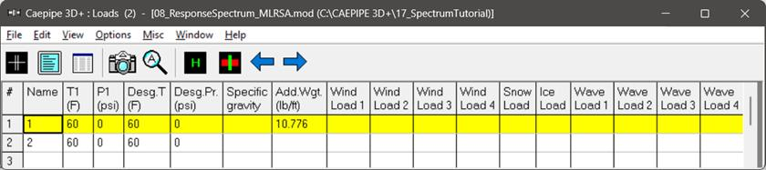
Once the inputting of different spectrums are done, input the Spectrum load itself for analysis through Layout window > Spectrum.

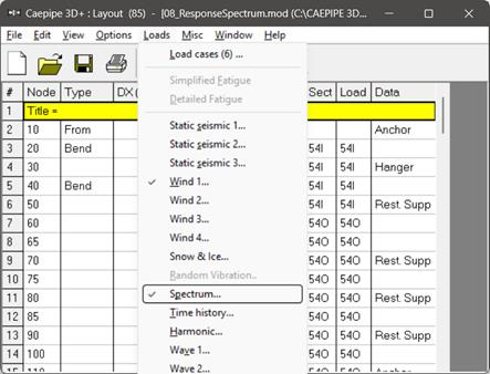
X, Y and Z spectrums

Select a spectrum from the drop-down combo box, which should have been input in the spectrum table for each direction.

Factor

The multiplying (scale) factor for the spectrum is input here. The same spectrum may be multiplied by different (Scale) factors to apply spectrum loads for different dynamic events. For example, vertical spectrum can be input as the same as that of the horizontal spectrum with a factor as shown above.

Mode Sum

Pick one of three choices, “SRSS” (square root of sum of squares), “Closely spaced” or “Absolute”.

Direction Sum

Pick one of two choices, “SRSS” (square root of sum of squares) or “Absolute”.

Step 4:

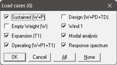
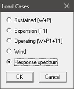
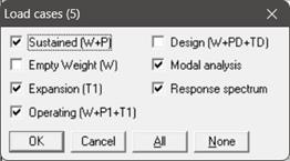
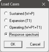
Turn ON the load case “Response spectrum” through Layout window > Loads > Load cases. Save the model and perform the analysis through Layout window > File > Analyze. CAEPIPE will apply these loads to compute the response of the piping system by performing a Response Spectrum analysis along with other load cases defined in the piping system.

Step 5:

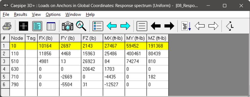
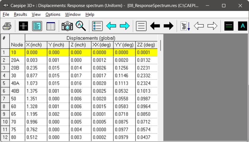
Upon analysis, CAEPIPE will show a “Load case” with name “Response spectrum” under “Support Loads”, “Displacements”, “Element forces” and “Support load summary” results.

Multi-level Response Spectrum Analysis

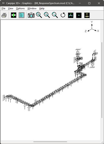
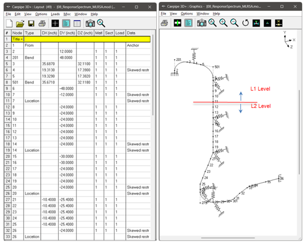
The model shown below is a 3 inch nominal diameter water line extending between two elevations, namely Level L1 and Level L2, with each Level experiencing different seismic loads. The layout has two anchors with a number of intermediate supports. The seimsic excitation consists of two separate spectra, with each spectrum corresponding to the two different Levels. All supports connected from node 1 through mode 11 (inclusive of the two end nodes) experience the upper level (Level L1) spectra excitation, while the remaining supports experience the lower level (Level L2) spectra excitation.

For this Multi-Level Response Spectrum Analysis, only the first 15 modes are used to approximate the response of the system. For each Level, the same spectrum load is applied along X, Y and Z directions with weighting factors of 1.0, 0.667 and 0.0 in the three global directions respectively.

The following are the Steps to perform the Multi-level Response Spectrum Analysis using CAEPIPE.

Step 1:

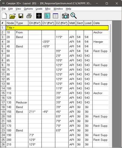
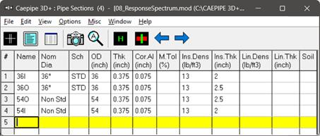
Attached is a sample CAEPIPE model with Response Spectrum. The piping layout shown below (extracted from the attached model “08_ResponseSpectrum_MLRSA.mod”) has the following layout and properties.

Step 2:

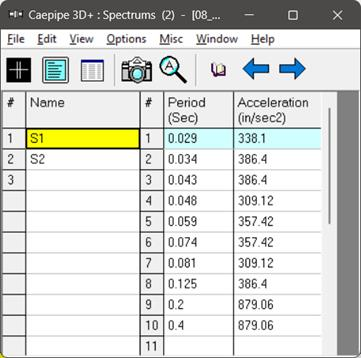
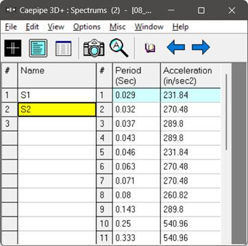
Input Spectrum load data from layout window: Misc Menu > Spectrums. This can be done in three ways:

1. Input spectrums directly into the model.

2. Create a spectrum library and load spectrums from it.

3. Input spectrums from a text file.

For further details, refer to the section titled “Spectrum Loads” in CAEPIPE User’s Manual.

When the first two methods are used, the units for the X-axis & Y-axis and the interpolation method are set through the Options > Spectrum.

Step 3:

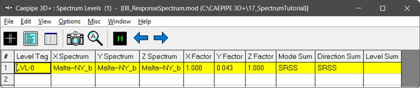
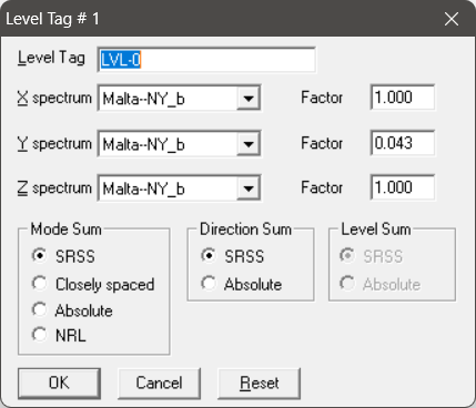
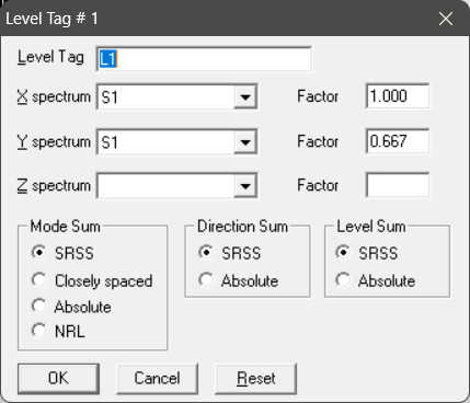
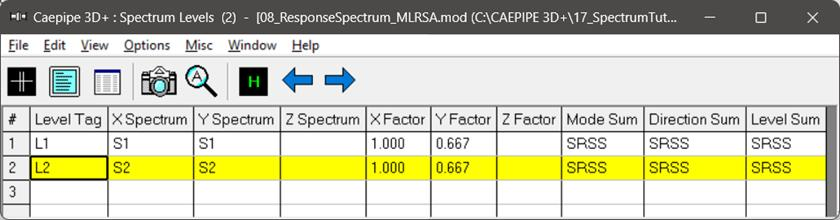
Define Spectrum Levels through Layout window > Loads > Spectrum. From the list window shown, double click on an empty row and input Level Tag, select Spectrums; input factors and select Mode Sum, Direction Sum and Level Sum. Levels L1 and L2 defined for this analysis are shown below.

Step 4:

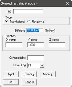
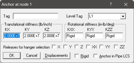
Assign Spectrum Level to each support in the analysis model by selecting the appropriate Level Tag from the list. Snapshots shown below are for a Restraint and an Anchor.

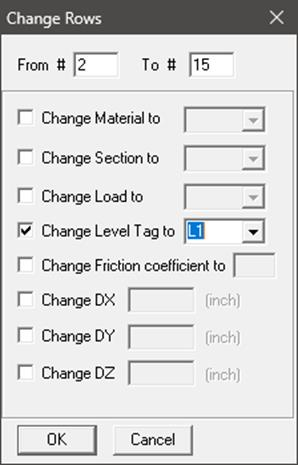
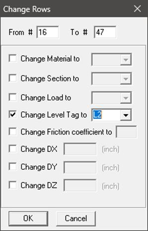
Alternatively, one can use the command “Change” through “Layout Window > Edit” to assign Level Tag for all supports in the Layout for a range specified as shown below.

Note:

The Level Tag selection list will be enabled and available for selection only when two or more Spectrum Levels are input in the analysis model. On the other hand, the Level Tag selection list will be disabled and the same Level Tag will be assigned automatically to all supports when only one Spectrum Level is defined in the analysis model.

Step 5:

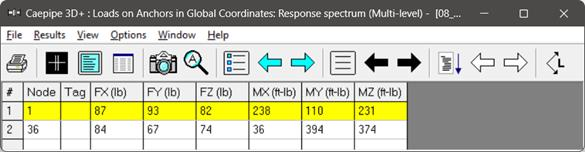
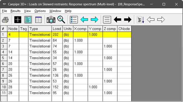
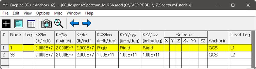
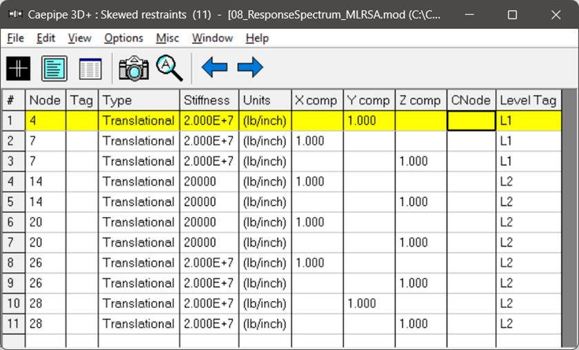
The users can review the Levels assigned to different supports using the List command. Snapshots shown below are from List command for Anchors and Skewed Restraints.

Note: CAEPIPE will terminate the analysis, if a level tag is not assigned to a support. For further details, refer to the flowchart under the section titled “Spectrum Loads” in CAEPIPE User’s Manual.

Step 6:

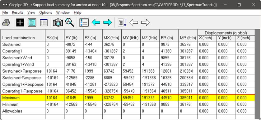
Upon analysis, CAEPIPE will show a “Load case” with name “Response spectrum” under “Support Loads”, “Displacements”, “Element forces” and “Support load summary” results.

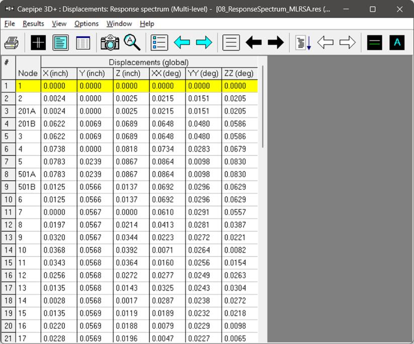
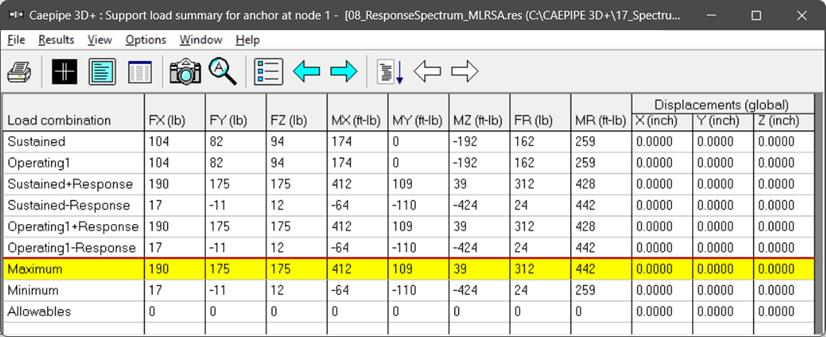
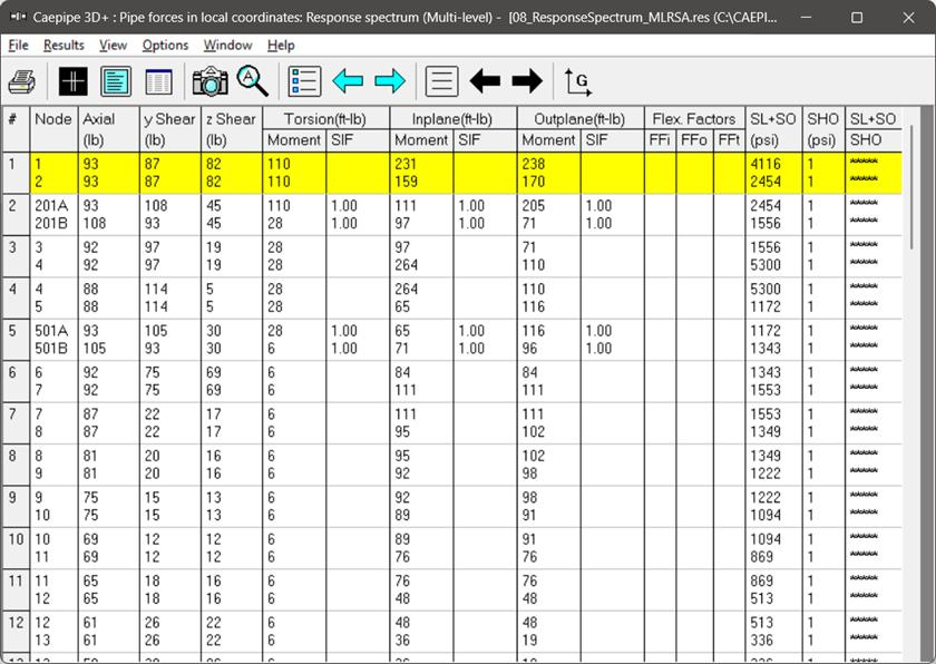
When selected, each results window (such as Support Loads, Displacements, etc.) will display the title as “Response Spectrum (Multi-level)” as shown in the snapshots below.