Tutorial on Fiber/Glass Reinforced Piping (FRP/GRP) Modeling and Analysis as per ISO 14692-3 using CAEPIPE
General
FRP pipes, also known as GRP pipes, fiberglass reinforced plastic pipes, is a type of conveying pipes with lightweight, high strength and corrosion resistance performance. The excellent corrosion resistance property and outstanding mechanical, physical and chemical performance save engineering, installation and maintenance costs, so it is regarded as the "user friendly" pipe.
FRP pipes have been proved to be superior to steel pipes in many aspects. They are widely used in industrial, civil engineering, petroleum, power and other fields.
FRP/GRP products are proprietary and the choice of component sizes, fittings and material types can be limited depending on the supplier. Potential vendors should be identified early in design to determine possible limitations of component availability.
FRP piping systems can be supported using the same principles as those for metallic piping systems.
In addition to the above, Buried FRP analysis requires computation of vertical soil load on pipe sections, live load on pipe due to the traffic and considers the effect of static overburden soil pressure.
This tutorial provides steps in performing piping stress analysis of both buried and above-ground FRP/GRP piping as per ISO 14692-3 using CAEPIPE.
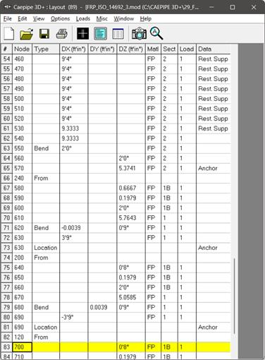
Snap shot shown below is a sample model for FRP/GRP Piping Analysis as per ISO 14692-3 where a portion of the layout is buried in soil (see the snapshot with RED highlight below) and the remaining portion of the layout is above the ground.


Step 1:
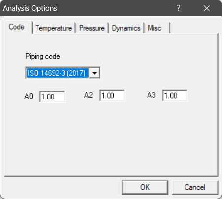
Select the piping code for analysis as “ISO 14692-3” through Layout Window > Options > Analysis > Code as shown below and press the button “OK”.
Step 2:
Next define FRP materials required for piping system through Layout window > Misc > Materials by obtaining their properties from the manufacturer or through the piping standard.
FRP Material Moduli
CAEPIPE requires three moduli for the FRP material:
· Axial or Longitudinal (this is the most important one)
· Hoop Modulus: If this modulus is not available, use axial modulus.
· Shear or Torsional: If this modulus is not available, use engineering judgment in specifying 1/2 of axial modulus or a similar value. Note that a high modulus will result in high stresses, and a low modulus will result in high deflections.
In the Material List window shown on the screen, double click on an empty row to input a new material or double click on a material description to edit the material properties.
In the Material dialog shown, enter the FRP material properties as given below.
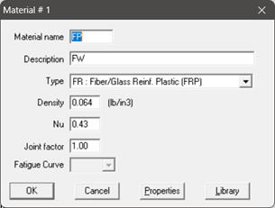
The material name can be up to five alpha-numeric characters. Enter description, density and Poisson’s ratio. You need to select “FR: Fiber Reinf. Plastic (FRP)” from the Type drop-down combo box before you click on the Properties button.
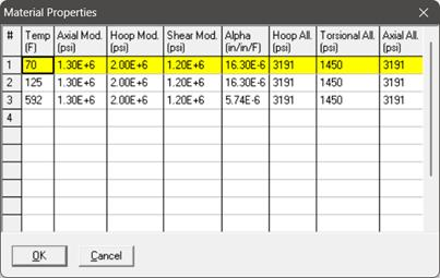
Step 3:
Click on the Properties button, you are shown the table below where you can enter temperature-dependent properties. Additionally, you can also define the Hoop, Torsional and Axial allowable stresses so that CAEPIPE can use them for code compliance checks as per ISO 14692-3 and display them under "Sorted FRP Stresses” results.
Step 4:
Define soils properties using the command Layout window > Misc > Soils.
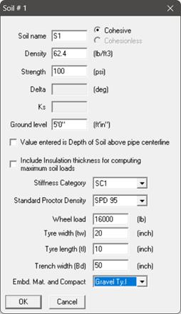
Two types of soils can be defined - Cohesive and Cohesionless.
Cohesive soil is hard to break up when dry, and exhibits significant cohesion when submerged. Cohesive soils include clayey silt, sandy clay, silty clay, clay and organic clay.
Cohesionless soil is any free-running type of soil, such as sand or gravel, whose strength depends on friction between particles. Cohesionless soil is not applicable for ISO 14692-3. Hence, the option is grayed out in the input screen.
Density is the density of the soil.
Strength
For cohesive soil, Strength is the same as Constrained modulus “Msn” defined in Table 5-6 of AWWA Manual M45 (second edition).
Ground Level
Ground level for a soil is the height of the soil surface from the global origin (height could be positive or negative). It is NOT a measure of the depth of the pipe’s centerline.
In the figure below, the height of the soil surface for Soil 1 is 3 feet from the global origin. Pipe node 10 [model origin] is defined at (0,-5, 0). So, at Node 10, the pipe is buried 8’ [= (3’ – (-5’)] deep into the soil. Define similarly for the other soil.
The pipe centerline is calculated by CAEPIPE from the given data.
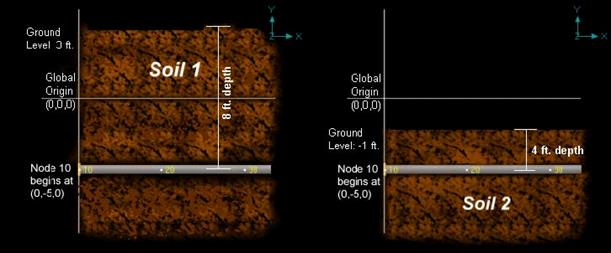
Depth of Soil above Pipe’s Centerline
When the option “Value entered is Depth of Soil above pipe centerline” is turned ON in Soil input, then CAEPIPE will compute maximum soil loads for the sections buried using the Depth entered. This option will be helpful for modeling pipes that are running up or down a hill with same depth of soil filled above pipe’s centerline as shown in the figure given below.

Warning:
Assign Soil only to those elements that are really buried in soil when the option “Value entered is Depth of Soil above pipe centerline” is turned ON.
Stiffness Category
Stiffness Category is required to compute the value of “Msb” the constrained soil modulus of the pipe zone embedment listed in Table 5-4 of AWWA Manual M45 (second edition). See the snapshot shown below.
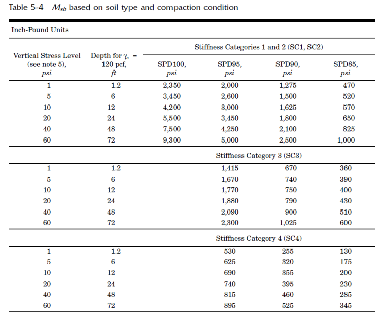
Standard Proctor Density
Standard Proctor Density is required to obtain the value of “Msb” (the constrained soil modulus of the pipe zone embedment) listed in Table 5-4 of AWWA Manual M45 (second edition).
Wheel Load
Value entered in “Wheel Load” field will be used to compute the Live Load (WL) on pipe. Refer to Sub-section 5.7.3.6 of AWWA Manual M45 (second edition). For example, the Truck Load field can be input as 16,000 lb for AASHTO-20 or 20,000 lb for AASHTO-25.
Tyre Width & Tyre Length
Tyre Width and Length input are used for computing the Live Load (WL) on pipe. By default, these values are set as 20” and 10” respectively. Refer to Sub-section 5.7.3.6 of AWWA Manual M45 (second edition) and Section “ISO 14692-3” in CAEPIPE Code Compliance Manual for further details.
Trench Width
Trench Width input is used to obtain the value of Sc from Table 5-5 which in turn is used for computing the maximum allowable vertical pipe deflection of pipe. Refer to Sub-section 5.7.3 and Table 5-5 of AWWA Manual M45 (second edition) and Section “ISO 14692-3” in CAEPIPE Code Compliance Manual for further details.
Step 5:
Tie the soils defined above with pipe sections through Layout window > Misc > Sections or Ctrl+Shft+S (to list Sections). Double click on the required section property. You will see the field Soil in the bottom right corner. Pick the soil name from the drop-down combo box.
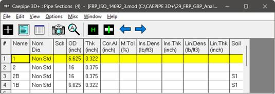
If a part of a piping system uses a certain pipe section with some portion of it buried and the balance not buried, then two separate sections have to be defined, with one of them without soil and the other with soil as shown above for Sections 2 and 2B.
Step 6:
Assign the appropriate section for each buried element on the Layout window with the correct soil around it.
Step 7:
Review the stress layout by highlighting the buried sections of the model in graphics. If your model contains sections that are above-ground and buried, then you can selectively see only the buried sections of piping in CAEPIPE graphics by highlighting the section that is tied to the soil. Use the Highlight feature under the Section List window and place highlight on the buried piping section (see Highlight under List window>View menu, or press Ctrl+H). The Graphics window should highlight only that portion of the model that is using that specific section/soil. See the portion shown in green in the figure below.

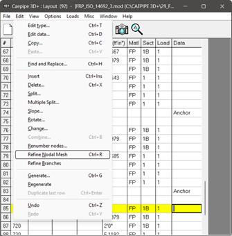
Step 8:
It is at the bends, elbows, and branch connections that the highest stresses are found in buried piping subjected to thermal expansion of the pipe. Hence, buried piping elements at the junction of bends, elbows and branch connections are to be refined in the stress layout.
This can be performed through Layout window > Edit > Refine Nodal Mesh > Buried Piping. Please see the section titled “Buried Piping” in CAEPIPE User’s Manual for details on “Nodal mesh generation”.

Step 9:
After completing the stress layout, save the model and analyze through Layout window > File > Analyze. See the file “FRP_ISO_14692_3.mod” available with this tutorials for further details.
Step 10:
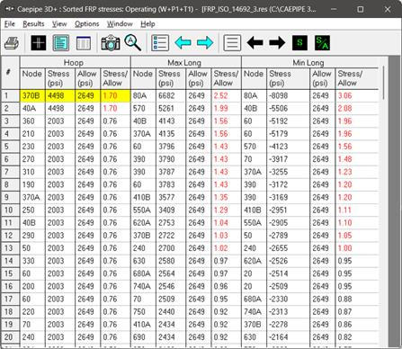
Upon successful analysis, CAEPIPE shows the code compliance as per ISO 14692-3 under Sorted FRP stresses as shown below.
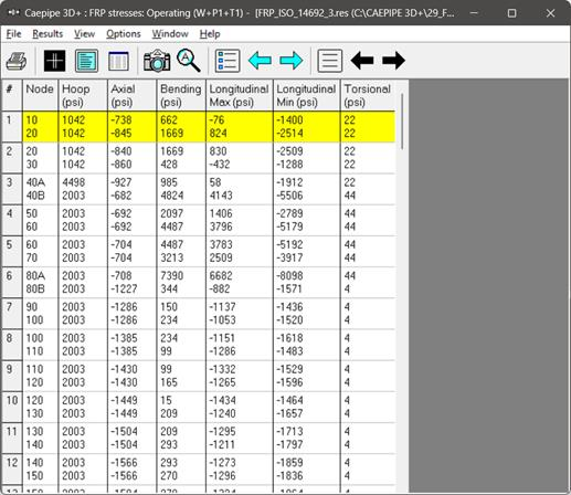
FRP stresses results of CAEPIPE display the stresses computed as per ISO 14692-3 on an element-by-element basis as shown below.
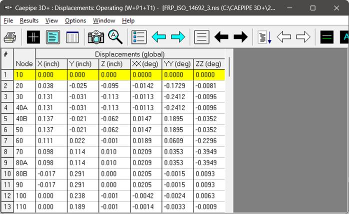
CAEPIPE will show the deflections and support loads for each load case under Deflections and Support loads results as shown below.
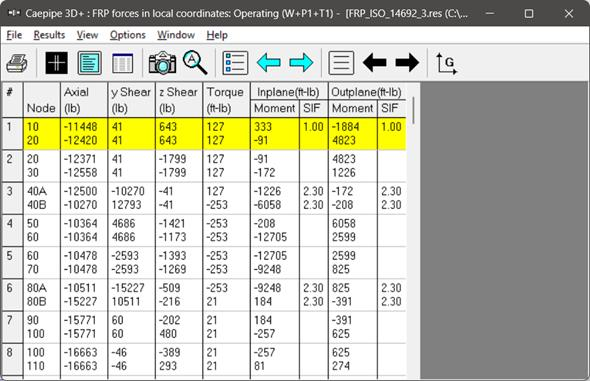
Element forces results for each load case (such as Sustained, Operating, etc.) show the Element forces and moments in local coordinate system along with Stress Intensification Factors (SIFs) computed as per analysis code ISO 14692-3 for each element as given below.
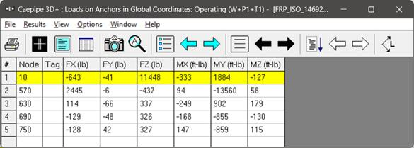
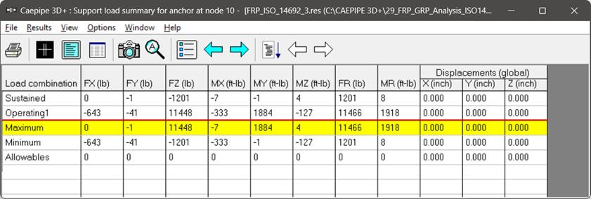
For the design of supports, Support Load Summary of CAEPIPE will show the loads on each support for all load cases selected for analysis as given below.
Stiffness matrix formulated internally in CAEPIPE is given below for quick reference.
Stiffness matrix
The stiffness matrix for a pipe is calculated using the following terms:
Axial term = L / EA
Shear term = shape factor x L / GA
Bending term = L / EI
Torsion term = L / 2GI
where L = length, A = area, I = moment of inertia, E = elastic modulus, G = shear modulus
For an isotropic material, G = E / 2(1 +  ), where = Poisson’s ratio,
For a FRP material, E = axial modulus and G is independently specified (i.e., it is not calculated using E and ).
).
The hoop modulus and FRP Poisson’s ratio are only used in Bourdon effect calculation where,
Poisson’s ratio used = FRP Poisson’s ratio input x (axial modulus / hoop modulus)
Note:
Refer to Section titled “ISO 14692-3” in CAEPIPE Code Compliance Manual of CAEPIPE for details on how CAEPIPE computes the Flexibility Factors, Stress Intensification Factors and Code Stresses as per ISO 14692-3.