Nonlinearities
There are several types of nonlinearities in CAEPIPE:
1. Gaps in limit stops and guides.
2. Rotational limits in ball and hinge joints.
3. Rod hangers as one-way restraints.
4. Tie rods with different stiffnesses and gaps in tension and compression.
5. Friction in limit stops, guides, slip joints, hinge joints and ball joints.
6. Buried piping.
An iterative solution is performed when nonlinearities are present. At the start of each iteration, the overall global stiffness matrix and the load vector are reformulated based on the solution (displacements) obtained from the previous iteration.
Limit stops with Gaps and Friction
Limit stops are input by specifying direction, the upper and lower limits (i.e., gaps) and optionally a friction coefficient and a support stiffness that comes into play when either gap is closed. The upper and lower limits are along the direction of the limit stop and measured from the undeflected position of the node. Typically, the upper limit is positive and the lower limit negative. The upper limit should be algebraically always greater than or equal to the lower limit. In some situations, it is possible to have a positive lower limit or a negative upper limit. If a particular limit does not exist (i.e., a node can move unrestrained in that direction), that limit should be left blank. If a gap does not exist, then the corresponding limit should be explicitly input as zero.
Solution Procedure
At the end of each iteration, the displacements computed at the limit stop node are resolved along the limit stop direction. The resolved displacement (in the limit stop direction) is compared with the upper and lower limits input for that limit stop. If the resolved displacement (in the limit stop direction) exceeds the upper limit or is less than the lower limit, the gap is closed; otherwise, it is open. The solution is converged when the displacements computed at the limit stop are within 1% of the corresponding displacements obtained at the end of the previous iteration.
If both upper and lower limits (gaps) of a limit stop are open, it is equivalent to having no limit stop and hence, no stiffness is applied at that limit stop node, and friction does not arise there.
If either one of the two gaps is closed (for example, in the case of most resting supports), the support load along the limit stop direction is calculated as [resolved displacement (in the limit stop direction) - gap distance] x user-specified stiffness for that limit stop. In this case, if friction is specified at the limit stop, the following iterative procedure is carried out.
1. The resultant displacement (d) in local yz plane is computed at this limit stop node.
2. The normal load at the limit stop is calculated as [resolved displacement (in the limit stop direction) - gap distance] x user-specified stiffness at that limit stop.
3. Using this calculated normal load, the friction force (ff) is calculated as ff = friction coefficient (mu) x normal load.
4. Using the friction force (ff) and the resultant displacement (d) in local yz plane, the equivalent friction stiffness (kf) is computed as kf = ff / d. Please note, if d is zero, then no friction force is computed, and hence, no equivalent friction stiffness is computed. If d is non-zero, then the following steps are carried out.
5. The global stiffness matrix is then updated to include the equivalent friction stiffness computed.
6. Analysis iteration is continued with the updated global stiffness matrix. The solution is converged when the displacements computed are within 1% of the corresponding displacements obtained at the end of the previous iteration.
7. After the solution has converged and if the gap is closed, the normal load and the friction force at the limit stop are calculated as:
Normal load at limit stop = [resolved displacement (in the limit stop direction) - gap distance] x user-specified stiffness for that limit stop.
y shear = fy = local y displacement x equivalent friction stiffness (kf)
z shear = fz = local z displacement x equivalent friction stiffness (kf)
Friction Force at Limit Stop = Resultant friction force (ff) = sqrt(fy^2 + fz^2)
During hanger design, the hot loads are recalculated with the status of the limit stops at the end of the preliminary operating load case. Then the hanger travels are recalculated using the recalculated hot loads.
In dynamic analysis, the status of the limit stops at the end of the first operating load case (W+P1+T1) is used. If either the upper or lower limit is reached for the first operating load case, the limit stop is treated as a rigid two-way restraint in the direction of the limit stop. If both limits are not reached, then that limit stop is treated as having no restraint.
Friction is specified by entering coefficient of friction for limit stop and guide, entering friction force and/or friction torque for slip joint, entering friction torque for hinge joint and entering bending and/or torsional friction torque for ball joint.
Friction is modeled using variable equivalent friction stiffnesses (fictitious restraints) in CAEPIPE as described in the above Solution Procedure. The stiffnesses of these fictitious restraints are estimated from the results of previous iteration. If friction is included in dynamic analysis, these equivalent friction stiffnesses computed from the last iteration of the first operating load case are included in modal and dynamic analyses.
Friction in Limit Stop
If the gap is not closed, there is no normal force and hence no friction. If the gap is closed, the normal force (limit stop support load) is calculated as explained above. The maximum friction force is friction coefficient * normal force. The resultant displacement (d) in local yz plane is computed at this limit stop node as explained above. Also let kf = equivalent friction stiffness which is assumed to be zero for the first iteration.
If d is non-zero then kf = maximum friction force / d
If kf > high stiffness ( 1×10¹² lb/inch) then kf = high stiffness [This is the case of no sliding]
In the next iteration the equivalent friction stiffness is added to the global stiffness matrix. The iterations are continued till the displacement ‘d’ in local yz plane is within 1% of displacement ‘d’ from the previous iteration. The friction force is d * kf.
Friction in Guide
A guide is modeled by adding high stiffnesses perpendicular to the direction of the pipe. The normal force in the guide is calculated by the vector sum of the local y and z support loads. Maximum friction force is friction coefficient * normal force. The displacements at the guide node are resolved in the direction of the guide axis. Let us call this displacement: x. Also let kx = equivalent friction stiffness which is assumed to be zero for the first iteration.
If x is non-zero or x * kx> maximum friction force,
then kx = maximum friction force / x
otherwise kx = high stiffness (1×10¹² lb/inch) [This is the case of no sliding]
In the next iteration the equivalent friction stiffness is added to the global stiffness matrix. The iterations are continued till the displacement x is within 1% of x displacement from the previous iteration. The friction force is x * kx.
The relative displacements (between From node and To node) for the slip joint are resolved in the direction of the slip joint. Let us call this relative displacement: x. Also let kx = equivalent friction stiffness which is assumed to be zero for the first iteration.
If x is non-zero or x * kx> friction force input,
then kx = friction force input / x
otherwise kx = high stiffness (1×10¹² lb/inch) [This is the case of no sliding]
In the next iteration the equivalent friction stiffness is added to the global stiffness matrix. The iterations are continued till the displacement x is within 1% of x displacement from the previous iteration. The friction force is x * kx.
Similar technique is used for friction torque (using rotations instead of translations).
Friction in Hinge Joint
The relative rotations (between From node and To node) for the hinge joint are resolved in the direction of the hinge axis. Let us call this relative rotation: x. Also let kx = equivalent friction stiffness which is assumed to be zero for the first iteration. Maximum friction torque = friction torque input + hinge stiffness input * x.
If x is non-zero or x * kx> maximum friction torque,
then kx = maximum friction torque / x
otherwise kx = high stiffness [This is the case of no sliding]
In the next iteration the equivalent friction stiffness is added to the global stiffness matrix. The iterations are continued till the relative rotation x is within 1% of x rotation from the previous iteration. The friction torque is x * kx.
Friction in Ball Joint
For a ball joint friction in bending (transverse) and torsional (axial) directions is treated independently. For the bending case, the resultant of the local y and z directions is used. Otherwise a procedure similar to the one used for hinge joint is used.
Friction in Dynamic Analysis
Friction is optional in dynamic analysis. Friction is mathematically modeled by using equivalent stiffnesses. If friction is included in dynamic analysis, these equivalent friction stiffnesses computed from the last iteration of the first operating load case are included in modal and dynamic analyses.
Misconvergence
During the iterative solution procedure for nonlinearities, a misconvergence is reported in the following manner:
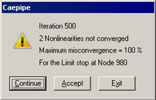
You have three options:
Continue the iterative procedure for 500 more iterations to see whether the solution converges, or
Accept the misconvergence (maximum misconvergence is reported, 100% in the above dialog), or
Exit the analysis processor completely.
An environment variable “CPITER” may be defined to change number of iterations from the default 500. For example, when “CPITER=1000”, iterations will continue up to 1000 before showing the dialog: Continue, Accept or Exit if there is misconvergence.
The shown misconvergence in the solution is really a quantification of how much off the results will be, IF you accept it. The maximum misconvergence (100% in the above case) is shown along with its location where such is happening.
In case of a solution with large misconvergence, you have two options: 1. Change parameters (mainly gaps and friction values, or removal of unneeded supports) inside the model to influence the convergence routine, or, 2. Increase the # of iterations. In case neither works, then use engineering judgment to accept or reject the merit of such a solution.