Relief Valve Load Analysis
General
During an overpressure event, the discharge of a PRV imposes a load, referred to as a reaction force, on the collective installation. The flowrate and associated reaction force increase from nominally zero to some value, remain relatively constant at that value for the duration of the release, and then decrease to zero again, i.e., when the relief valve opens, the discharge fluid creates a jet force that acts on the piping system. This force increases from zero to its full value over a time frame similar to the opening time of the valve. The relief valve remains open until sufficient fluid is vented to relieve the overpressure situation. As the valve closes, the reduction in flow reduces the jet force to zero.
Simplified Analysis Approach
American Petroleum Institute’s API 520, Part II (1994), provides a basis for calculation of the reaction force in the event of a vapor or a two-phase release directly to the atmosphere. There is no discussion in this section of API 520, Part II, about the reaction force developed during a liquid release. Furthermore, no guidance is presented with respect to applying these results or determining if an installation is acceptable; instead, the burden is placed on the designer to ensure that the installation is appropriately designed. While this may be reasonable for the design of new facilities, evaluating the adequacy of existing facilities becomes much more complicated.
The formula (section 2.4.1.1) in US Customary units from API 520, Part II (1994), for vapor relief devices discharging to the atmosphere, is shown below:
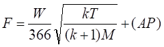
where,
F = Reaction force at the point of discharge to the atmosphere,(lbf.)
k = Ratio of specific heats (CP/CV) at the outlet conditions
W = Flow rate of any gas or vapor, pound mass (lbm.)/hr
CP = Specific heat at constant pressure
CV = Specific heat at constant volume
T = Temperature at the outlet, °R
M = Molecular weight of the process fluid
A = Area of the outlet at the point of discharge, in2
P = Static pressure within the outlet at the point of discharge, psig
Using the reaction force computed from the above formula along with the following PRV parameters, namely
· Valve Opening Time,
· Valve Closing Time and
· Relief duration (all obtained from the PRV manufacturer),
One can generate a PRV load profile and apply it in CAEPIPE to perform a simplified analysis.
Detailed Analysis Approach
Section 2.4.2 of API 520, Part II (1994) also states the following.
“Pressure relief devices that relieve under steady-state flow conditions into a closed system usually do not create large forces and bending moments on the exhaust system. Only at points of sudden expansion will there be any significant reaction forces to be calculated. Closed discharge systems, however, do not lend themselves to simplified analytical techniques. A complex time history analysis of the piping system may be required to obtain the true values of the reaction forces and associated moments.”
Such complex time history analysis of the piping system can be carried out as follows.
· Perform a fluid transient analysis on the piping system using a fluid dynamics software tool such as, “PipeNet”, “RELAP”, "ROLAST", etc.
· Apply the resulting output obtained (forces as a function of frequency) at the bend node after the relief valve in a pipe stress analysis software (CAEPIPE).
· Compute forces, moments and stresses in the piping system due to this loading.
As one can see, this method is detailed, time consuming and expensive and hence, not covered here.
Example 1:
Step 1:
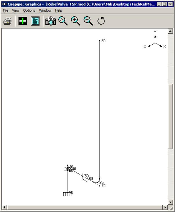
By assuming the following data, one can apply the relief valve loading in CAEPIPE. Please see the model below for details.
1. Reaction force (F) computed using the formula above = 6854 lb.
2. Relief Valve Opening time = 8 ms (milliseconds)
3. Relief Valve Closing time = 8 ms
4. Relief duration = 1 s
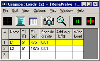
6. Pressure = 475 psig
7. Temperature = 51°F
The steps followed in generating the model are given below.
Step 2:
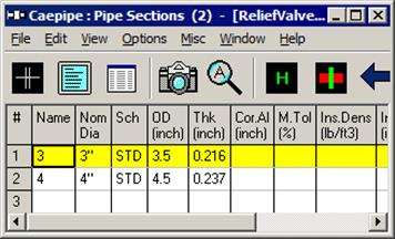
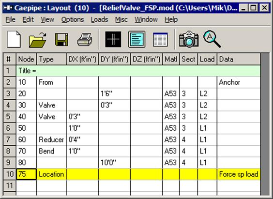
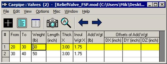
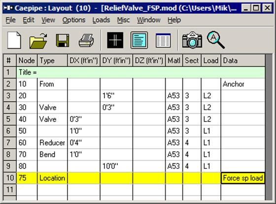
After creating your piping model (with node 75 being the center node of the discharge bend where the PRV reaction force will be applied),
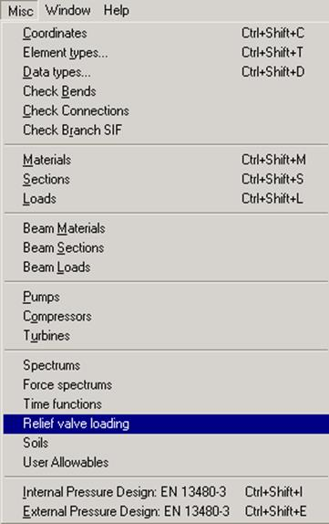
Select “Relief valve loading” from CAEPIPE Layout window > Misc and enter the data in the dialog box as shown in the figure below.
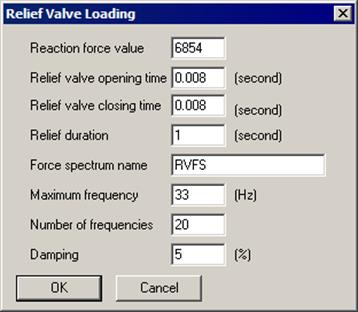
Step 3:
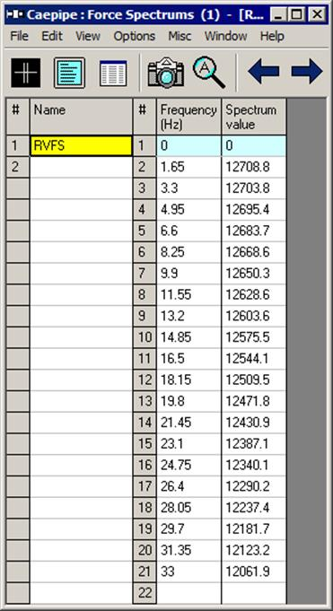
After entering the data as shown in the dialog above, press the button “OK”. Using the above input values for Relief Valve Loading, CAEPIPE internally generates a time-history loading function, which is then applied on a single degree-freedom spring-mass system with each intermediate frequency (between 0.0 Hz and the maximum frequency) to generate the “Force Spectrum Load” shown below.
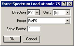
Step 4:
Apply the Force Spectrum Load thus generated at the bend center node 75 after the relief valve in downward direction (-FY by specifying negative Scale Factor) as shown below.
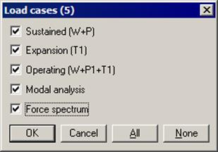
Step 5:
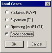
Check “Force Spectrum” for analysis through Layout window > Load cases. Click on OK.
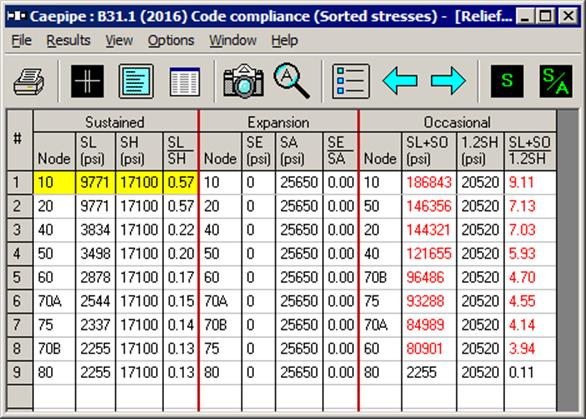
Step 6:
Save and Analyze the model. After analysis, CAEPIPE displays Occasional stresses which include the effects of the PRV load.
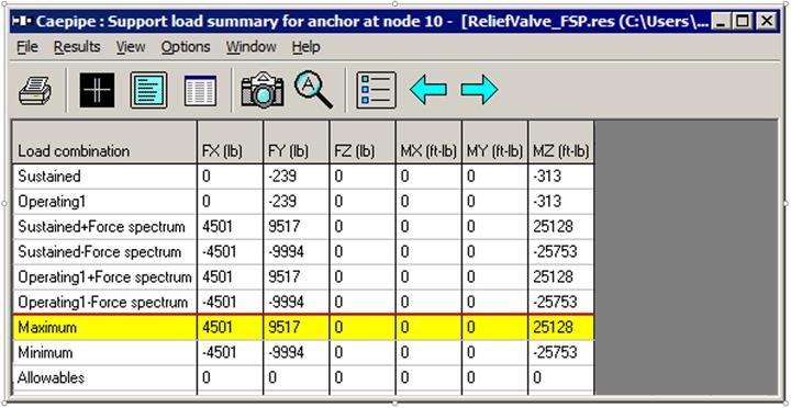
Step 7:
Another load case called “Force Spectrum” will be available for which you can study displacements, support loads, support load summary (for sizing supports), etc.