Wave Load
You can enter up to four (4) wave load data namely Wave Load 1, Wave Load 2, Wave Load 3 and Wave Load 4.
You can apply a wave load to the whole or parts of the model. To apply the wave load to the required portion of the layout, input "Y(es)" under the Layout Window > Misc > Loads > Wave Load 1/Wave Load 2/Wave Load 3/Wave Load 4. When done, CAEPIPE internally computes wave load for each element and applies it as a lumped load (i.e., concentrated force) equally at the two nodes of each element (i.e., it is not a distributed load along the element).
When an element is subjected to a wave load, CAEPIPE computes forces due to Drag, Inertia and Lift due to Horizontal particle Velocity, Current Velocity and Horizontal particle Acceleration as well as Drag, Inertia and Lift due to Vertical particle Velocity and Vertical particle Acceleration. The forces thus computed are considered in Occasional load case.
Apart from the above, the element is also subjected to Buoyancy force. At present, this buoyancy force is computed using the properties input under Wave Load 1. This effect reduces the apparent weight of the piping as it acts against the gravity. Hence, the Buoyancy effect is included in Sustained load case.
Drag and Inertia forces generally act in the direction of the wave velocity and Lift force will be normal to the direction of the wave velocity. For example, when the wave direction is parallel to Global Z with Vertical axis being parallel to Global Y, then the Drag and Inertia forces will act in Global Z direction and Lift force will be in the plane normal to Global X and Global Z directions (i.e., parallel to Global Y direction). For further details, refer to the Section titled “Wave Load” in CAEPIPE Code Compliance Manual.
The dialog for specifying wave load is given below.
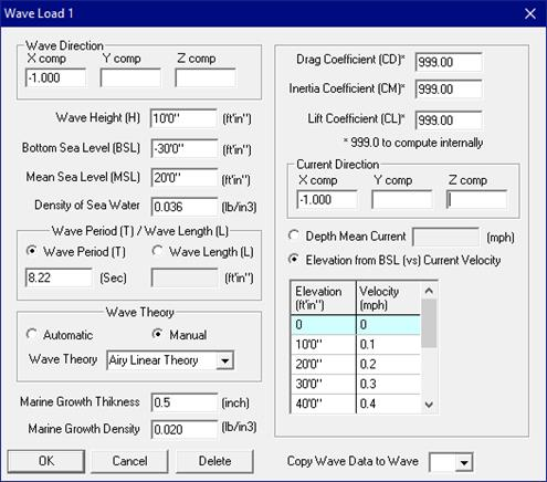
Wave Direction
Input the direction of the wave using the direction cosines (for example: When the vertical axis is parallel to Global Y, for wave in Z direction, X comp = 0.0, Y comp = 0.0, Z comp = 1.0; for wave in 45° X-Z plane, X comp=0.707, Y comp=0.0, Z comp=0.707). See section titled “Direction” in this Manual. CAEPIPE will allow inputting the wave direction only in the horizontal plane and NOT in the vertical direction.
Mean Sea Level and Bottom Sea Level
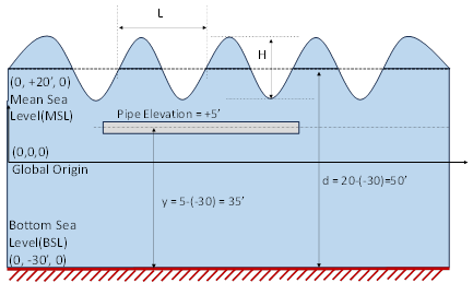
Mean Sea Level (MSL) is the distance of the mean water surface from the global origin (it could be positive or negative). It is NOT a measure of the depth of the pipe’s centerline.
In the figure below, the distance of the water surface is 20’ feet above the global origin. The horizontal pipe starts at, say, (10, 5, 0). So, the pipe is submerged 15’ (= 20’ - 5’) below the Mean Sea Level into the water.
Similarly, Bottom Sea Level (BSL) is the distance of the sea bed level from the global origin (it could be positive or negative). In the figure, the distance of the sea bed is -30’ feet below the global origin. So, the pipe is located at a distance of 35’ feet from the Bottom Sea Level. This is indicated as “y” (pipe centerline from BSL) in the figure.
Wave Depth (d) is computed as the difference between the Mean Sea Level and Bottom Sea level (i.e., d = MSL – BSL). So, in the figure below, d = 20 – (-30) = 50’0”.
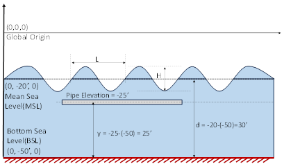
Given below is another example, wherein the global origin is above the Mean Sea Level (MSL).
Density of Sea Water
Input the density of Sea Water. Seawater density varies depending on temperature, salinity, and pressure. The average density of ocean is about 1030 kg/m3.
Wave Period / Wave Length
Input one of the following: wave period (sec) or wave length (ft or mm). Depending upon the Wave Theory selected, CAEPIPE will internally compute the other parameter using the dispersion relation. For example, if you input the wave period, CAEPIPE will automatically calculate the wavelength (or vice versa) based on the selected wave theory (either chosen manually or determined automatically when the 'Wave Theory' option is set to 'Automatic').
Wave Theory Selection
User can select the Wave Theory Manually or instruct CAEPIPE to determine the appropriate Wave Theory by selecting the option “Automatic”.
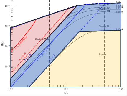
When the option “Automatic” is selected, then CAEPIPE computes the Ursell (UR) parameter using the wave parameters input in the dialog along with the chart given below to decide the Wave Theory. Ursell parameter is defined as UR = HL2/d3, where d = Wave Depth as explained above, H = Wave Height and L = Wave Length.
1. “Airy’s Linear Theory” when UR < 1.00 and H/L < 0.0064. This region is shown in YELLOW in the below chart.
2. “Stokes 5th Order” when the UR computed internally is within the BLUE region shown below in the chart, and
3. “Cnoidal 5th Order” when the UR > 26.0 and within the RED region shown below in the chart.
Note 1:
In cases where the “Automatic” option is turned on and CAEPIPE selects ‘Stokes 5th Order’ or ‘Cnoidal 5th Order’ theory based on the Ursell parameter, but the selected theory does not converge, then CAEPIPE automatically switches to the ‘Fenton Fourier Stream Function’ theory with an appropriate order selected internally to ensure a stable and accurate solution.
Note 2:
If Wave Length required for computing the Ursell parameter is not input, then CAEPIPE computes the Wave Length by solving the dispersion relation as per Airy’s Theory using Wave Period.
Wave Theory
The following wave theories are available for manual selection or will be automatically chosen by the program when the 'Wave Theory' option is set to 'Automatic'.
1. Airy’s Linear Theory
2. Stokes 5th Order
3. Cnoidal 5th Order
4. Fenton’s Fourier Stream Function Theory
5. Dean-Dalrymple Stream Function Theory
6. Solitary Wave Theory
Airy’s Linear Theory
The Airy’s linear wave theory is the simplest and most useful theory among various wave theories. It assumes small wave steepness (H/L) and small relative water depth (H/d), which allows the free surface boundary conditions to be linearized and satisfied at the Mean Sea Level (also known as Still Water Level, SWL).
Stokes 5th Order
The Stokes wave theory assumes that the velocity potential and water free surface level as power series in terms of a non-dimensional small perturbation parameter  which is defined as the product of wave number and wave amplitude. Stokes 5th Order theory considers power series until 5th order. Stokes wave theory is most useful when the depth to wave length ratio, d/L is greater than 1/10.
Cnoidal 5th Order
Finite amplitude long waves of permanent form in shallow water are better described by the Cnoidal wave theory. The Cnoidal wave is a periodic wave that usually has sharp crests separated by wide troughs. The theory accounts for a large class of long waves of finite amplitude. The approximate range of validity of the theory is d/L < 1/8 and the Ursell parameter,  . Note that the Ursell parameter is defined as UR = HL2/d3.
Fenton Fourier Stream Function Theory
The Fenton Fourier Stream Function theory represents nonlinear waves using a Fourier series expansion of the free surface elevation and velocity potential, with the governing free-surface boundary conditions satisfied iteratively. Unlike classical stream-function formulations, the free surface is explicitly described through Fourier coefficients, providing direct control over the wave profile. The theory is applicable over a wide range of water depths and wave conditions, including steep and highly nonlinear waves. It is particularly useful when high accuracy and spectral representation of wave kinematics are required, and for verification against classical nonlinear wave solutions.
Dean-Dalrymple Stream Function Theory
The Dean-Dalrymple Stream Function theory represents nonlinear wave motion by expressing the flow field using a stream function expanded in a Fourier series, with the free surface treated implicitly as a streamline. The governing equations and nonlinear free-surface boundary conditions are satisfied through an iterative solution procedure. This theory is suitable for finite water depths and can model strongly nonlinear waves, including cases with constant-vorticity shear currents. It is widely used in engineering practice due to its numerical robustness and reliable convergence for nonlinear wave and wave-current interaction problems.
Solitary Wave Theory
Solitary wave theory represents the limiting case of extremely shallow water waves, consisting of a single crest entirely above the still water level with no trough. It is applicable when (water depth/wavelength) d/L → 0 (i.e., the wavelength is very long relative to the water depth) and the Ursell number is very high. This theory is commonly used for modeling tsunamis, tidal bores, and waves very close to shore, where the wave behaves as an isolated pulse of energy translating without change of form. It can be considered as the limiting case of cnoidal theory when the elliptic parameter m → 1.
Note:
For the Fenton Fourier Stream Function theory and the Dean–Dalrymple Stream Function theory, the user is provided with an option to specify the order of the Fourier series or stream-function expansion. The order can be selected within a range of 1 to 32, allowing control over the level of accuracy and resolution of the computed wave kinematics. Higher orders generally improve the representation of nonlinear wave profiles but may increase computational effort. For all other wave theories, this option is not applicable and is therefore disabled (grayed out).
To apply any of the theories listed above, enter the required parameters for the wave. CAEPIPE uses these parameters along with the dispersion relation to determine the wave length or wave period.
After calculating the wave length (L) and/or wave period (T), CAEPIPE determines the horizontal and vertical particle velocities (u & v), as well as the horizontal and vertical particle accelerations (du/dt & dv/dt), for various phase angles (from 0 to 180 degrees) at the pipe centerline elevation, referenced from the bottom sea level. These velocity and acceleration values at each phase angle are then used in Morison’s equation (in both horizontal and vertical directions) to compute the maximum concentrated forces due to Drag, Inertia and Lift in the three global directions (FX, FY and FZ) at each node.
A few Technical articles, Text books and other documents referred for the implementation of wave theories for wave loading in CAEPIPE are listed at the end of this section.
Marine Growth Thickness and Density
The effect of accumulation of algae, sea weed, coral, etc., surrounding the pipe can be considered in the analysis by specifying the Marine Growth Thickness and Density. Marine Growth leads to the increase in Outer Diameter of the piping thereby affecting the Buoyancy, Weight of the piping and Wave Kinematics. In addition, when you input a non-zero value for Marine Growth Thickness in the dialog, then CAEPIPE considers the pipe surface as “Rough” while determining the Drag, Inertia and Lift coefficients. On the other hand, when the Marine Growth thickness is input as 0.00 or left BLANK, then CAEPIPE considers the pipe surface as “Smooth” while computing these coefficients.
Drag, Inertia and Lift Coefficients
The Drag Coefficient (CD) represents the resistance encountered by the body due to the flow of fluid (viscous effects). The Inertial Coefficient (CM) captures the accelerative impact of wave forces generated by the pressure field around the body. The Lift Coefficient (CL) indicates the normal force perpendicular to the flow, arising from phenomena like vortex shedding and asymmetric flow patterns.
Any of the coefficients can be entered in the following ways:
· Non-zero positive value: Applied to all elements selected for the wave analysis, considering both horizontal and vertical fluid velocities and accelerations.
· +999.0: CAEPIPE computes the corresponding coefficient internally and applies it to the elements selected, considering both horizontal and vertical fluid velocities and accelerations.
· Non-zero negative values: The absolute value of the coefficient entered will be used, but only horizontal fluid velocities and accelerations are considered (vertical components are excluded).
· -999.0: CAEPIPE computes the value internally and applies it to the elements selected, but only horizontal fluid velocities and accelerations are considered (vertical components are excluded).
· Zero (0.0): The effect of that force is ignored entirely in the analysis (e.g., setting CD to 0.0 ignores Drag force).
Current Data (Direction and Current Velocity)
User can input the direction and current velocity to be included in the analysis. The current velocity can be input either as “depth mean current” (current velocity independent of depth) or as a function of elevation with respect to Bottom Sea Level.
Generally, current direction is parallel to the wave direction. However, CAEPIPE has the option to input any direction for the current in the Horizontal plane. In such cases, CAEPIPE computes the Drag and Lift forces accordingly.
References
[1]. American Petroleum Institute. (2000). Recommended Practice for Planning, Designing, and constructing Fixed Offshore Platforms – Working Stress Design (API RP 2A-WSD, 21st Edition). Washington, D.C.
[2]. Sarpkaya, T., & Isaacson, M. (1981). Mechanics of wave forces on offshore structures. Van Nostrand Reinhold
[3]. Airy, G. B. (1845). Tides and waves. In Encyclopaedia Metropolitana (Vol. 5, pp. 241–396). London: Richard Griffin & Company.
[4]. Chakrabarti, S. K. (1987). Hydrodynamics of Offshore Structures. WIT Press.
[5]. Skjelbreia, L., & Hendrickson, J. (1960). Fifth-order gravity wave theory. In Proceedings of the 87th Coastal Engineering Conference (Chapter 10). Den Haag.
[6]. J. D. Fenton (1990). Nonlinear Wave Theories. The Sea, Vol.9: Ocean Engineering Science, Eds. B. Le Méhauté and D.M. Hanes, Wiley, New York.
[7]. Morison, J. R., O'Brien, M. P., Johnson, J. W., & Schaaf, S. A. (1950). The force exerted by surface waves on piles. Petroleum Transactions, AIME, 189, 149–154.
[8]. Dean, R. G., & Dalrymple, R. A. (1991). Water wave mechanics for engineers and scientists. World Scientific.
[9]. DNV GL. (2016). DNVGL-ST-0437: Loads and site conditions for wind turbines. DNV GL AS.