Tutorial for Modeling and Results Review - Problem 1
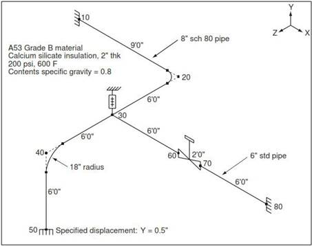
The best way to learn CAEPIPE is to try it yourself. In this tutorial we will create a simple model to help you understand the use of CAEPIPE. The details of the model are shown below:
You will learn how to:
1. Enter Title
2. Select Analysis options (piping code etc.)
3. Define Material, Section and Loads for the model
4. Input Model Layout
5. Select Load Cases for Analysis
6. Analyze
7. View Results
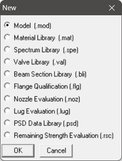
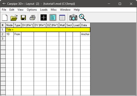
From the “New file” dialog, select the type of the new file as “Model (.mod)” file. This opens two independent windows: “Layout” and “Graphics”.
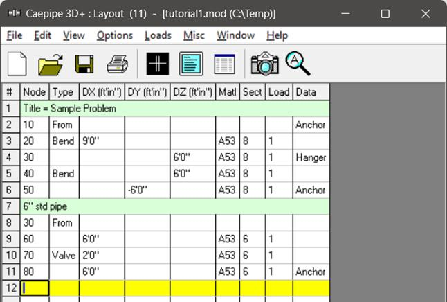
Layout window
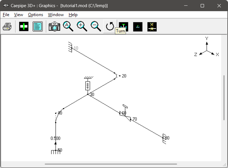
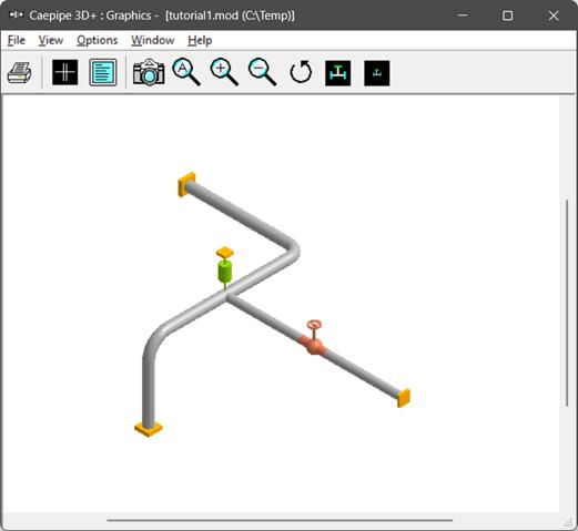
Graphics window
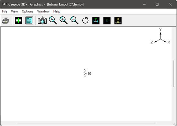
Adjust the size of the windows to fit your desktop such that you can view both comfortably at the same time.
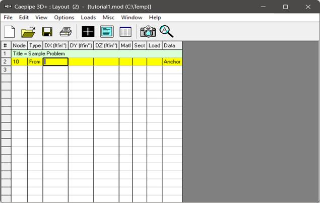
1. Enter Title
Type “Sample Problem” as the title in the first row that contains “Title =”. Press Enter.
2. Select Analysis options (piping code etc.)
Click on the “Options” menu and then select “Analysis” (Options > Analysis) to specify options for analysis.
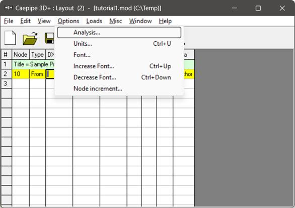
This opens the “Analysis” Options dialog.
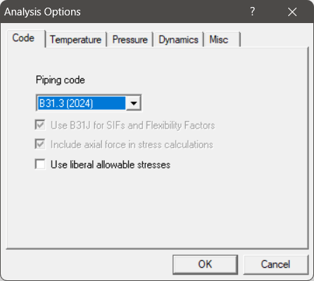
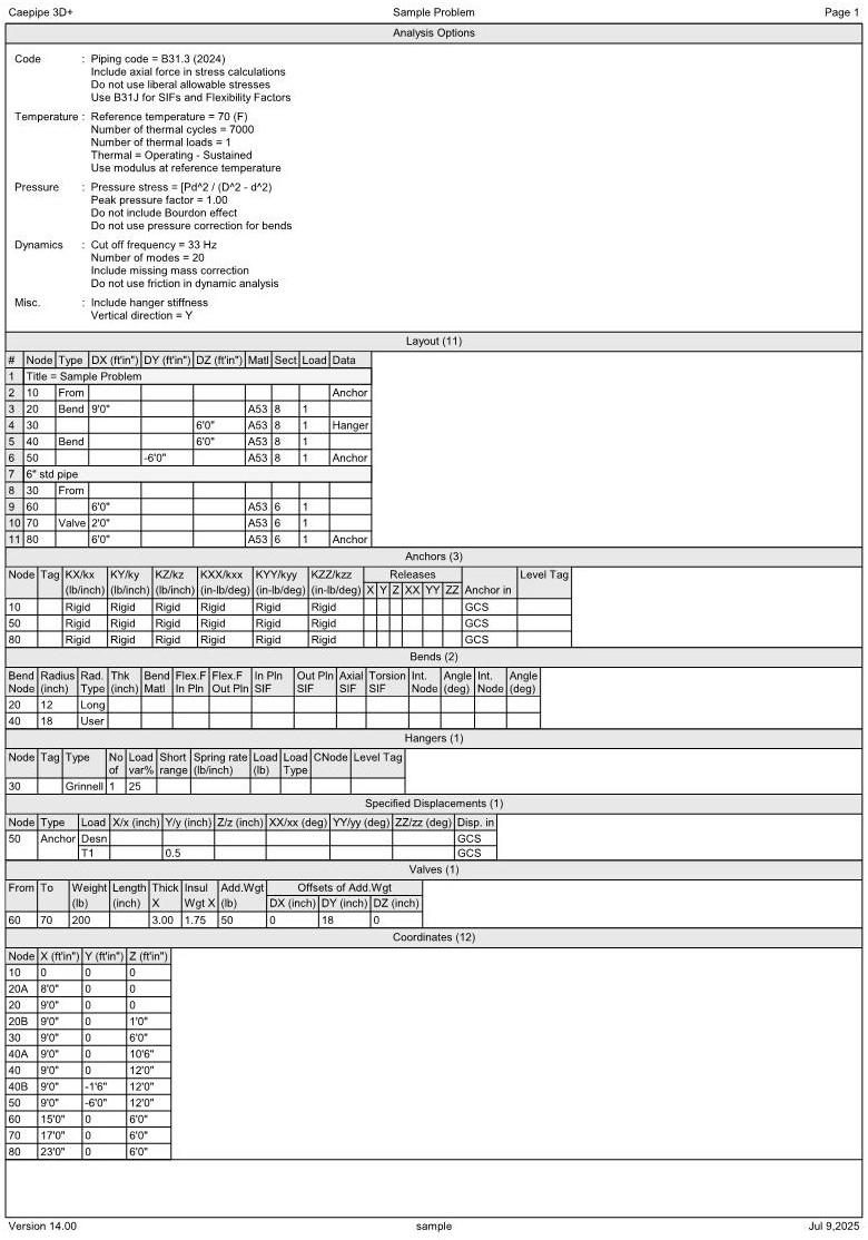
On the Code property page, select “B31.3 (2024)” for Piping code. Then click on “OK” to close “Analysis Options” dialog.
3. Define Material, Sections and Load Material
Click on “Matl” in the header in the Layout window (or press “Ctrl+Shift+M”)
This opens up the “Materials” list in a separate “List” window. Position and resize the list window as you desire. Click on “Library” button on the “Toolbar” (or choose File > Library).
The “Open Material Library” dialog is shown
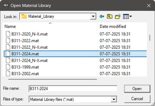
Select “B313-2024.mat” as the library file to open by double clicking on it. The available materials in the library are shown.
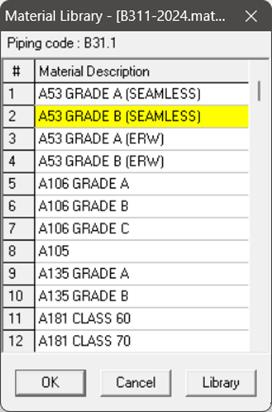
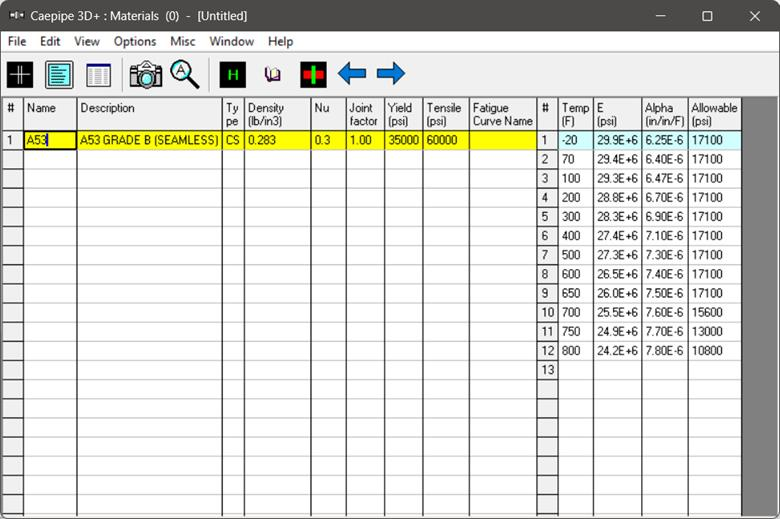
Double click on “A53 Grade B (SEAMLESS)” material to select it. The properties for this material are transferred to the material in the List window. Type “A53” for material name and then press “Enter”.
Sections
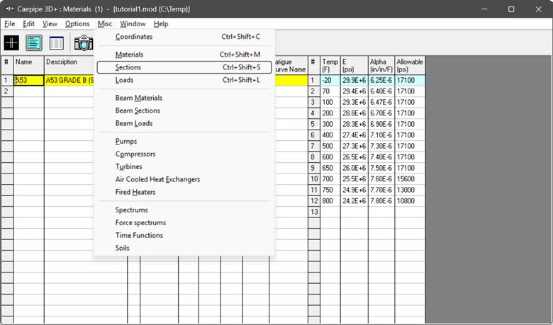
Select “Sections” from the “Misc” menu of the List window (or press “Ctrl+Shift+S”).
The “Sections” list is shown. To enter the first section, Type “8” for section name and press “Enter”. The Section Properties dialog is shown with the section name 8.
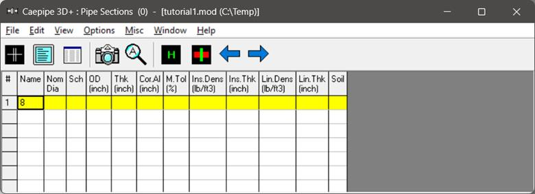
The Section Properties dialog (“Section #1”) is shown with the section name 8.
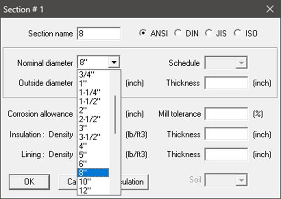
Click on the “down arrow” of the “Drop Down” combo box for “Nominal diameter” and select 8” for “Nominal diameter”. The “Outside diameter” (8.625”) is automatically entered.
To select the schedule for the 8” pipe, click on the “down arrow” of the “Drop Down” combo box for “Schedule” and select 80 for “Schedule”.
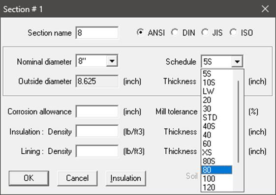
The “Thickness” (0.5”) is automatically entered.
For “Insulation density”, click on the “Insulation” button or Press “Alt+I”.
A table of “Insulation materials and their densities” is shown.
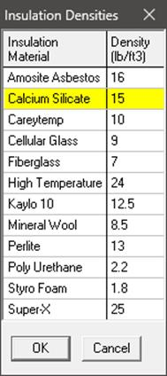
Double click on “Calcium Silicate”. The “Insulation density” (15.0 lb/ft3) is entered on the “Section” dialog. Type 2 (inches) for “Insulation Thickness” then press “Enter” or click “OK” to enter the first section.

Now repeat the process for the second section.
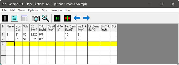
In row # 2, type 6 for section “Name” and press Enter. The “Section Properties” dialog is shown with the section name “6”. Select 6” for “Nominal diameter”, STD for “Schedule” and 2” Calcium Silicate for “Insulation”. Press “Enter” or click on “OK” to enter the second section.
Load
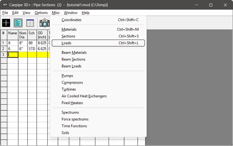
Select “Loads” from the “Misc” menu (or press “Ctrl+Shift+L”).
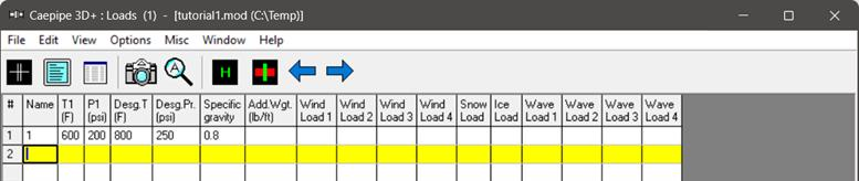
The “Loads” list is shown. To enter the first load, Type “1” for “Name”, Tab to “T1” and type 600, Tab to “P1” and type 200, Tab to “Desg. T” and type 800, Tab to “Desg. Pr.” And type 250 and Tab to “Specific gravity” and type 0.8. Then press “Enter”. That is it! The load is entered. (Alternately, you could have pressed “Ctrl+E” on the first row and typed in the same information in a dialog box).
Note:
Design Temperature and Design Pressure should always be greater than or equal to the Operating Temperature and Operating Pressure (T1 and P1 for this tutorial).
Design Temperature entered will be used to compute the allowable stress for material while computing the Allowable Pressure as per the piping code selected.
The Allowable Pressure computed as per the piping code selected is then compared against the Design Pressure entered above and reported in the Code Compliance results.
In addition to the above, starting “CAEPIPE V.12.10”, there is an additional load case for Design Pressure and Design Temperature that computes and show results for “Displacements”, “Element Forces” & “Moments”, “Support Loads” and “Support Load Summary”.
Click in the Layout window or press F3 to move the focus to the Layout window.
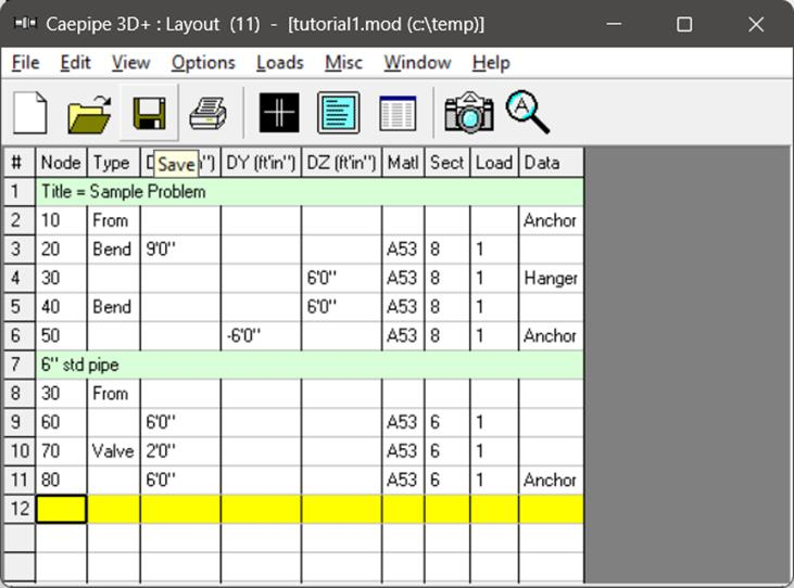
4. Input Model Layout
We are going to model the 8” header line first, followed by the 6” branch line.
Note:
· In the following text, the word “type” should be distinguished from the words “Type column” or simply “Type” (upper case “T”). The former (“type”) would mean press the keys for the text you want to type. The latter word “Type” would refer to the Type column in the Layout spreadsheet.
· Also, the instruction “type B for Bend” does not necessarily mean the upper case “B”. The lower case “b” could also be typed.
· For items input in the “Data” column (such as “Anchor” or “Hanger”), the cursor needs to be in the “Data” column. This can be quickly done by pressing Ctrl+D from any column or clicking in the “Data” column. Another way is to Tab repeatedly to reach the “Data” column.
· As the graphics window is simultaneously updated, you should position the graphics window in such a way that you can see it along with the input window.
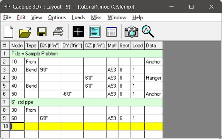
First the 8” header
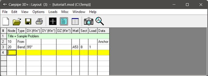
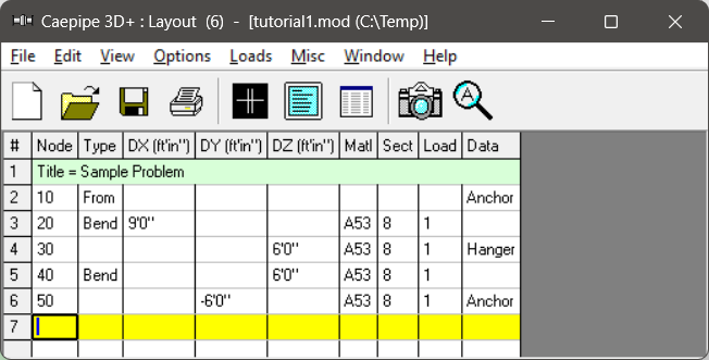
Following the “Title” at row #1, row #2 is already generated with “Node” 10 of Type “From” with an “Anchor” in the “Data” column.
Press “Enter” to move the highlight to the next row #3. Tab to the “Type” column. The next “Node” 20 is automatically assigned. In the “Type” column, type “b” (for Bend), Tab to “DX”, type 9. Tab over to “Material”, type A53, Tab to “Section”, type 8, Tab to “Load”, type 1. Press “Enter” and the cursor moves to the next row (#4).
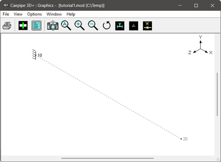
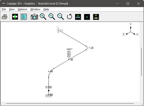
You will see the model in the graphics window as it is entered. You can press “F2” to switch between text and graphics windows.
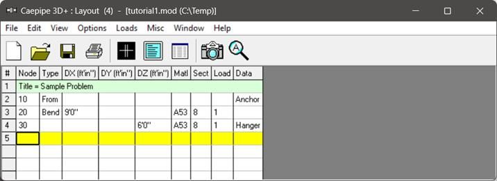
In row #4, Tab to the “Type” column. The next “Node” 30, is automatically assigned.
In row #4 with “Node” 30, Tab to “DZ”, type 6, Tab to “Data” (or press “Ctrl+Shift+D”), type “h” (for a to be designed Hanger) and press “Enter”, the “Hanger” dialog is opened.
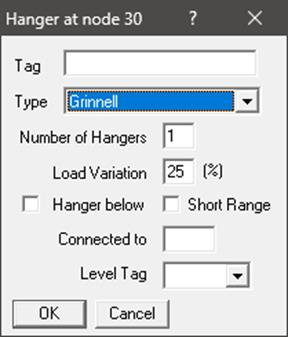
Press “Enter” or click on “OK” to input the hanger. The material, section and load are automatically inserted (based on the previous row’s material, section and load), and the cursor moves to the next row.
The Graphics window will look like this.
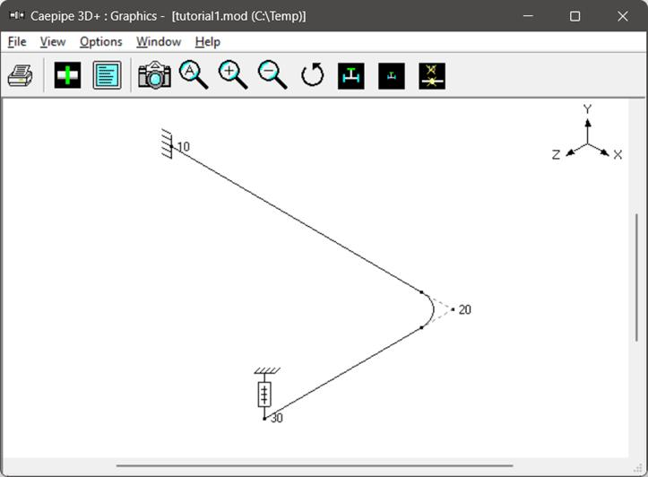
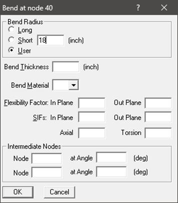
In row #5, Tab to the “Type” column. The next “Node” 40, is automatically assigned. In the “Type” column, type “b” (for “Bend”) and press Tab. This bend has a non-standard (user defined) bend radius. Therefore, the bend radius needs to be modified from the default long radius. Double click on the “Bend” in the “Type” column or press “Ctrl+T” to bring up the “Bend” dialog box. Click on “User” (Bend Radius > User) radio button and enter 18 for “Bend Radius”. Press “Enter” or click on “OK” to modify the bend.
While still in row #5, Tab to “DZ”, type 6 then press- “Enter”. The material, section and load are automatically inserted like before, and the cursor moves to the next row.
In row #6, Tab to the “DY” column. The next “Node” 50, is automatically assigned. In the “DY” column, type -6, Tab to the “Data” column or press “Ctrl+Shift+D” to move to the data column, then type “a” (for “Anchor”). Anchor, material, section and load fields are automatically inserted, and the cursor moves to the next row.
Let us specify a thermal anchor movement for the “Anchor” we just put in at node 50. Double click on the “Anchor” at node 50 in row #6. The “Anchor” dialog comes up.
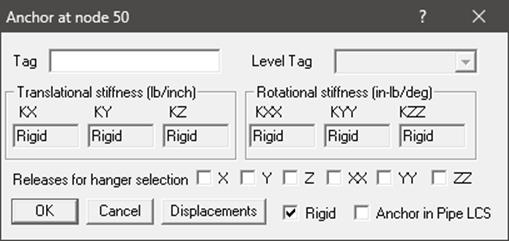
Note:
Option “Anchor in Pipe LCS” allows the user to input Anchor stiffnesses in the “Local Coordinate System” (LCS) of the adjoining pipe. On the other hand, if “Anchor in Pipe LCS” is not turned ON, then the user has to input Anchor stiffnesses in the “Global Coordinate System” (GCS).
Click on “Displacements” button. The “Specified Displacements” dialog for the anchor comes up. Tab to “Y” displacement field and type 0.5.
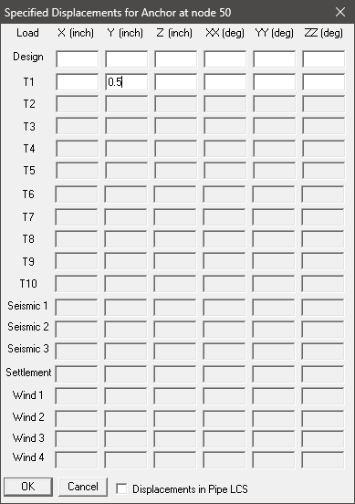
Press “Enter” to exit the “Specified Displacements” dialog. Press “Enter” again to exit the “Anchor” dialog. In the “Layout” window, press “Enter” to move to the next row.
Now the 6” branch
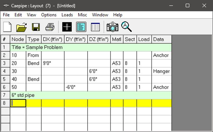
Let us input a comment saying that this is a 6” std pipe. On an empty row, if the first character in the Node field is input as “c”, that row becomes a comment row. On row #7, type “c” to create the comment and then type: “6” std pipe” and then press “Enter” to go to the next row.
On the next row (#8), type 30 for Node, Tab to the “Type” column, type “f” (for “From”, since we are beginning a new branch), press “Enter”. In the next row (#9), Tab to the “DX” column. The next “Node” 60 is automatically assigned. In the “DX” column, type 6 and press “Enter”.
CAEPIPE inserts the previous material, and automatically detects the new branch and asks if you want to change section.
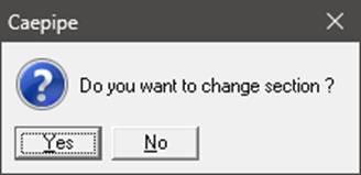
Since we want to change the section to 6, click on “Yes”. This opens the “Select Section” dialog.
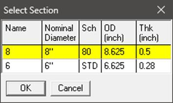
Select the 6” section by double clicking on it. The section (6) is entered in the “Section” column in the “Layout” window. Press “Enter” to go to the next row. The load is again automatically inserted from the previous load.
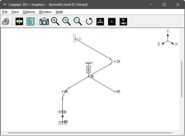
The graphics window will look like this.
In the next row (#10), Tab to the “Type” column. The next “Node” 70, is automatically assigned. In the “Type” column, type “v” (for “Valve”). This brings up the “Valve” dialog box.
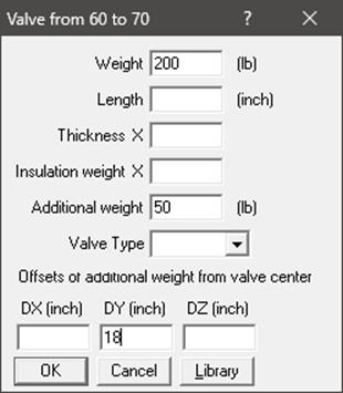
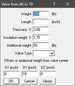
In the “Valve” dialog box, type 200 for “Weight”, 50 for “Additional Weight” and 18 for “DY” offset. Then press “Enter” or click on “OK” to input the valve. The “Thickness X” and “Insulation weight X” are automatically added as 3.00 and 1.75 by CAEPIPE as shown.
In the Layout window, type 2 for “DX” offset and press “Enter”. The material, section and load are automatically inserted as before, and the cursor moves to the next row.
In the next row (#11), Tab to “DX”. The next “Node” 80 is automatically assigned. In the “DX” column, type 6. Tab to “Data” or press “Ctrl+Shift+D” to move to the data column, then type “a” (for “Anchor”). Material, section and load are automatically inserted like before, and the cursor moves to the next row.
5. Select Load Cases for Analysis
Select “Load cases (4)” from the Loads menu.
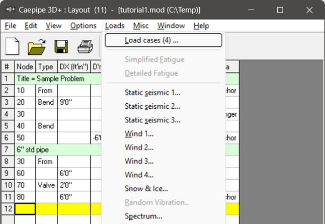
The “Load cases” dialog is shown.
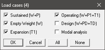
By default, “Sustained” (W+P), “Empty Weight” (W), “Expansion” (T1) and “Operating” (W+P1+T1) load cases are already selected. “Design” (W+PD+TD) load case when selected for the “Analysis”, CAEPIPE will compute and show results for “Displacements”, “Element Forces & Moments”, “Support Loads” and “Support Load Summary”. A design load case does not include “Stress Calculations”, “Rotating Equipment Qualifications” and “Flange Equivalent Pressure Calculations”. Press “OK” to return to the “Layout” window. The model input is now complete.
List
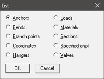
Click on an item of interest to show the list for that item. A list of all the anchors in the sample model is shown below:
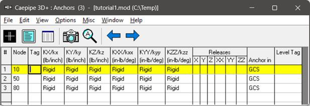
The highlighted item can be edited directly in the “List” window (in most cases) or in a dialog by pressing “Ctrl+E”. The items can be deleted by pressing “Ctrl+X”. The item is also highlighted in the graphics window by flashing and with a box around the node number.
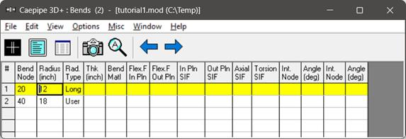
A list of all the bends in the sample model is shown below:
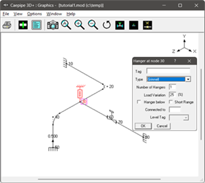
Editing in the Graphics Window
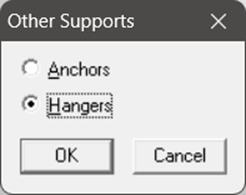
Another useful feature is the ability to edit an item in the graphics window. When an item such as a “Hanger” is clicked in the graphics window, a dialog box for that item is opened, where it can be modified.
The “Save Model As” dialog is shown.
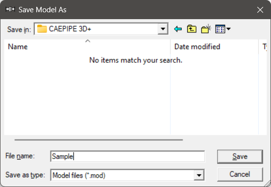
Type the File name as “Sample” and press Enter to save the model. We are done with modelling. Let us analyze now.
6. Analyze
Click on “Analyze” under the File menu.
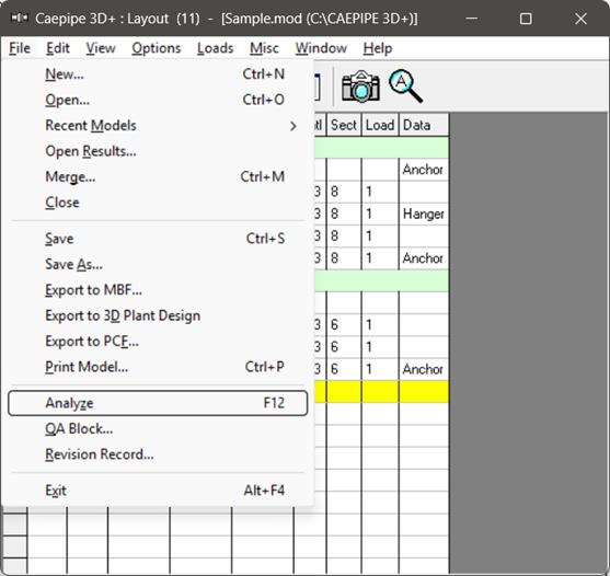
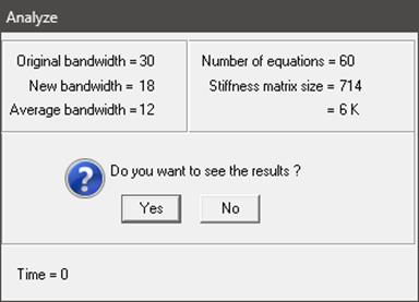
After the analysis, you are asked if you want to see the results. Select “Yes”.
7. View Results
After finishing the analysis and choosing to see the results or by opening the results file (.res), the results window is displayed. The “Results” dialog is opened automatically.
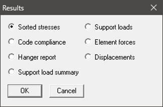
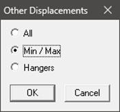
Select an item of interest by clicking on it. When you are viewing the results, use Tab (or “Next Result” button) to view the next result and “Shift+Tab” (or “Previous Result” button) to view the previous result. The “Results” dialog can be brought up by clicking on the “Results” button (or press “Ctrl+R”).
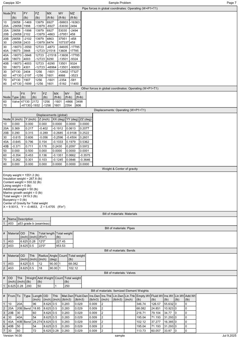
While viewing the results, the model data can also be simultaneously viewed in separate “Layout” and “List” windows. These are now “read only” windows, i.e. the model data cannot be modified while viewing the results. Some of the results from the sample problem are shown below:
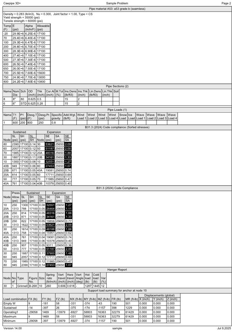
Sorted Stresses
The computed stresses (“sustained”, “expansion” and “occasional”) are sorted in descending order by stress ratios.
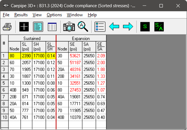
When the stress ratio exceeds 1.00, the stress and the stress ratio are shown in red. In this particular case, the high thermal stresses may be reduced by replacing the anchor at “Node” 80 by a guide. This allows the 6” pipe to expand more freely and reduce the thermal stresses. The maximum thermal stress is reduced to 22784 psi and the stress ratio is reduced to 0.77.
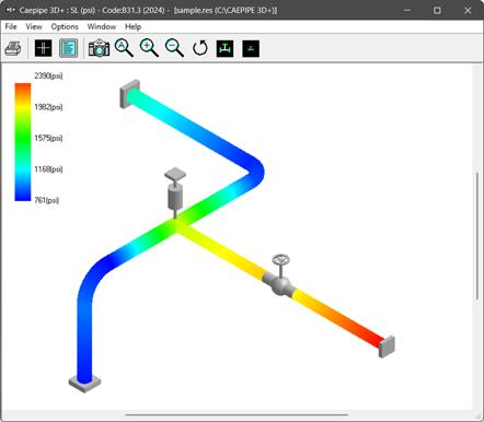
Instead of rendering color coded stresses/ratios, the values of stresses/stress ratios may be plotted by using the menu: “View > No color coding”.
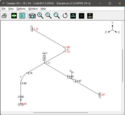 0
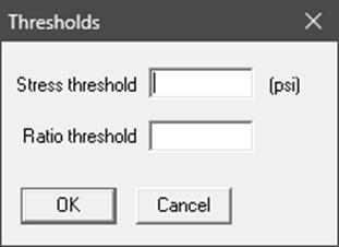
0While plotting stresses or stress ratios, thresholds may be specified (choose “View > Thresholds”). Only the stresses or stress ratios exceeding the thresholds are plotted.
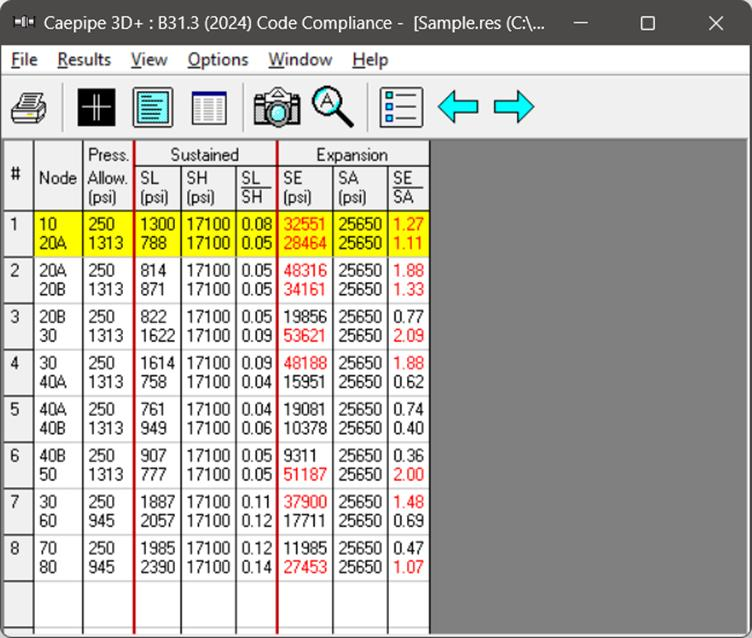
Code compliance
The element stresses and stress ratios calculated according to the piping code are shown under “Code Compliance”. Design pressure and CAEPIPE calculated “Allowable pressures” are shown in 2nd column.
Hanger report
The hanger report is shown below.
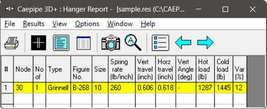
The “No of” field shows the number of hangers required at the indicated location. The “Figure No.” and “Size” refer to the manufacturer’s catalog. The vertical travel (also referred to as “Hanger travel”) is the vertical deflection at the hanger location for the first operating load case. Similarly, the horizontal travel is the resultant horizontal deflection at the hanger location for the first operating load case. The hot load is the hanger load at the operating condition and the cold load is the hanger load at zero deflection.
Variability (%) = (Spring rate × Hanger travel / Hot load) × 100
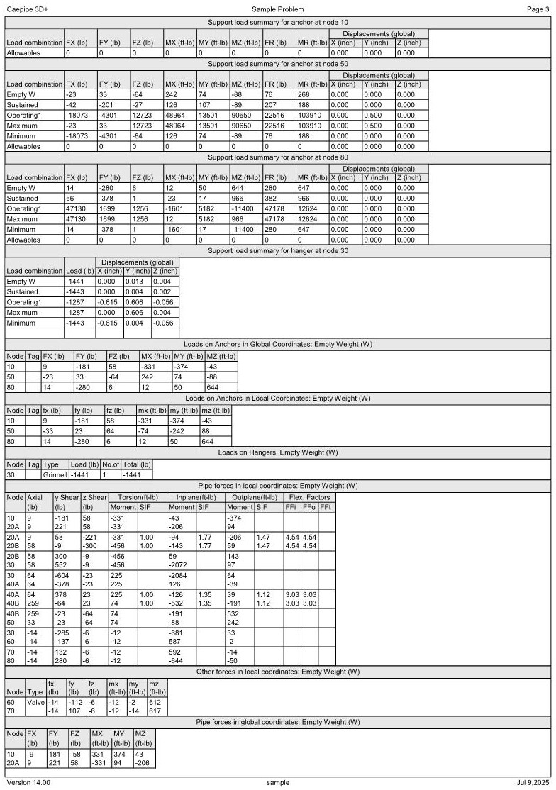
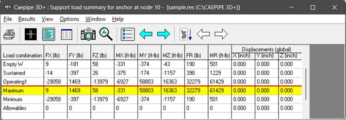
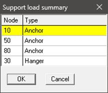
Support load summary
“Support load summary” for each support is created by considering all the load cases and appropriate combinations and then showing the maximum and minimum loads.
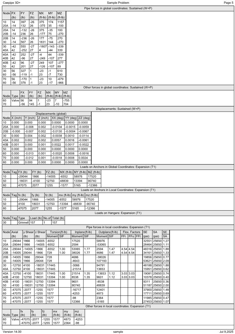
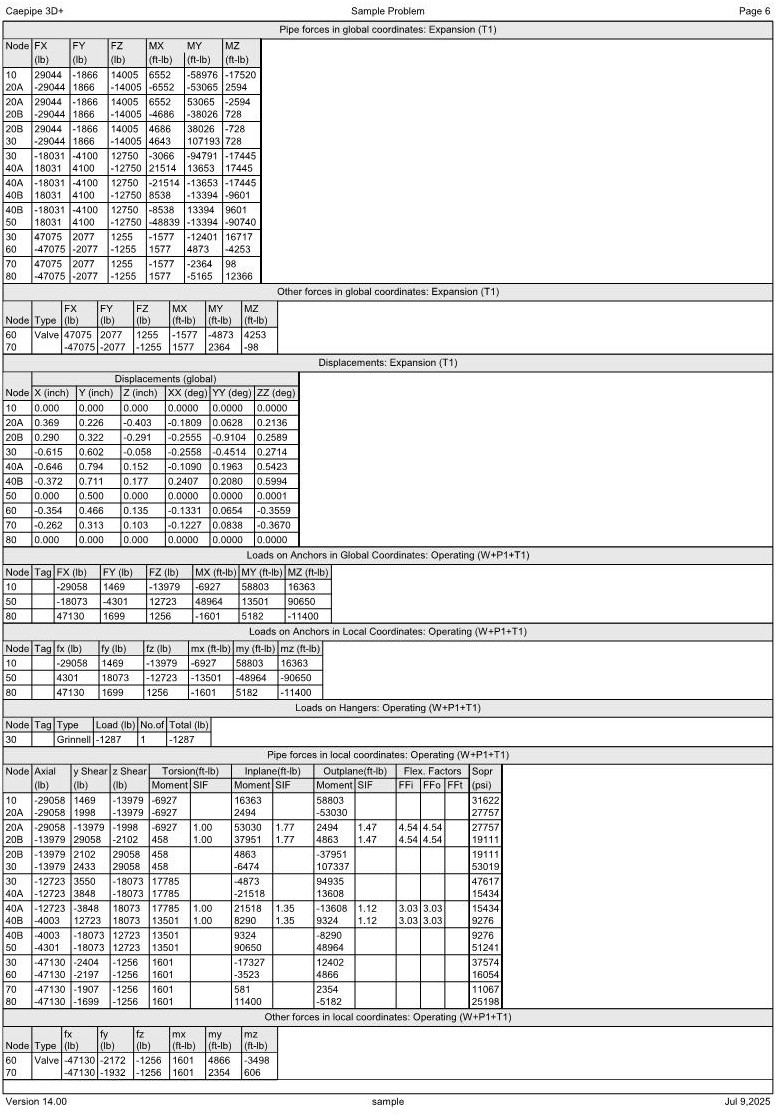
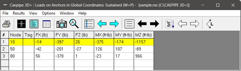
Support loads
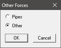
Support loads are the loads acting on the supports by the piping system for the selected load case. The loads on anchors for the “Sustained” case are shown below.
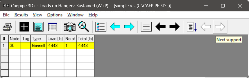
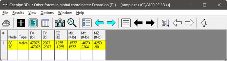
For example, the loads on hangers (i.e. the loads acting at the hanger locations imposed by the piping system) for the “Expansion” case are shown below.
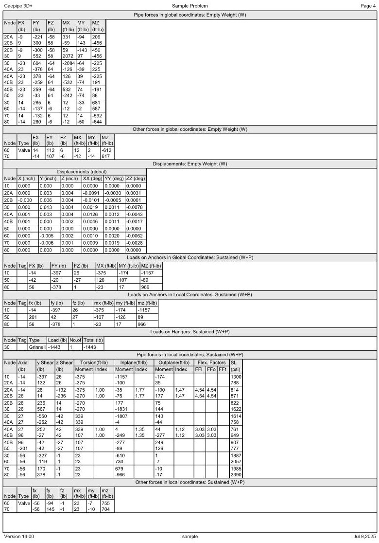
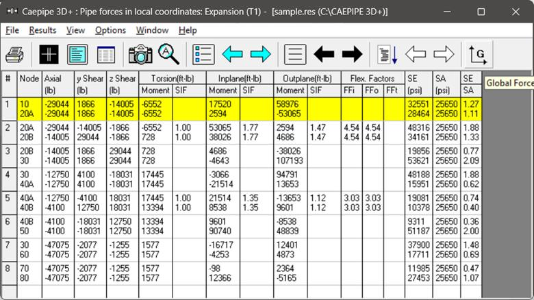
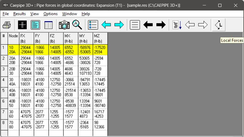
Element Forces
For pipe (also bend and reducer), element forces in local coordinates, “Stress Intensification Factors” (SIF), “Flexibility Factors” (FF) and stresses are shown by default for the selected load case.
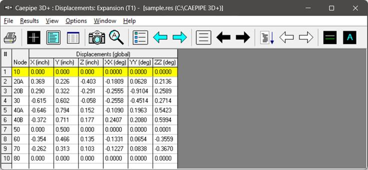
Displacements
The nodal displacements are shown.
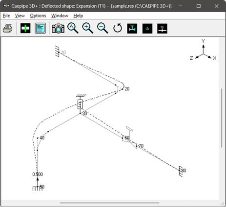
Choose “View > Magnification” to change the magnification of the deflected shape.
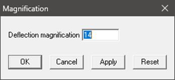
The reset button is used to calculate a default magnification factor which scales the maximum deflection to about 5% of the width of the graphics window.
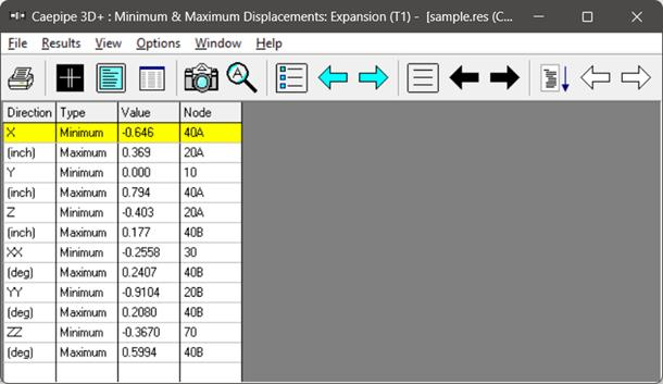
The minimum and maximum displacements for each of the directions and the corresponding nodes are shown below.
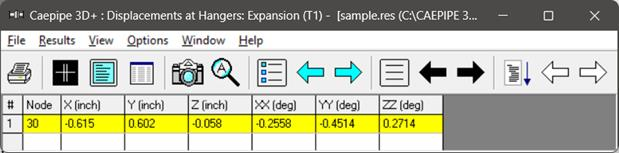
The displacements at hanger nodes are shown below.
Print
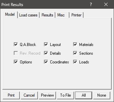
You can also print to a text file by using the “To File” button. A preview of the printed output can be seen by using the “Preview” button.
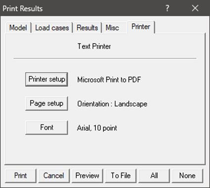
The printing options such as choice of printer, margins, portrait or landscape and font can be set on the Printer tab.
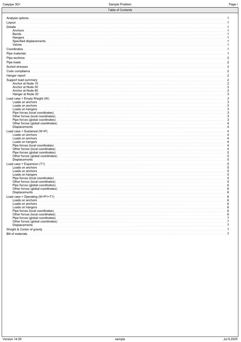
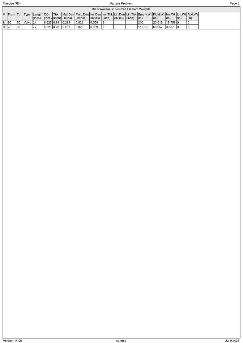
The sample problem report is shown next. Observe that for sorted stresses and code compliance, when the stress ratio exceeds 1.00, the stress and the stress ratio are shown in white letters on black background.
This is the end of the tutorial. If you have questions or comments, please email them to:
support@sstusa.com.