Tutorial for Modeling and Results Review - Problem 2

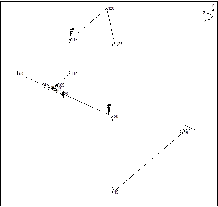
Let us model a slightly more advanced piping system now that you have familiarized yourself with the basic use of CAEPIPE via Tutorial 1. The details of the model (in SI units) are shown below:

You will learn how to:

1. Enter Title

2. Select Analysis options (piping code etc.)

3. Deﬁne Material, Section and Loads for the model

4. Input Model Layout (different loads for different segments)

5. Select Load Cases for Analysis

6. Analyze

7. View Results

Model Description

Details of the Layout, Material, Sections, Loads and Connection details are summarized for reference:

1. Axes Chosen: Global X = East, Global Y = Up and Global Z = South

2. Piping Code: ASME B31.1 (2024)

3. Section Properties:

a) Main Line: 10” Schedule STD

b) Branch Line: 6” Schedule STD

4. Insulation throughout the Piping system:

a) Density: 176.2 kg/m3

b) Thickness: 65 mm

5. Material: A 312 TP 316

6. Temperature:

a) For Main Line and Branch Line up to Valve End Node 105:

b) Operating Temperature = 185 Deg. C and Design Temperature = 230 Deg. C

c) For Branch Line after Valve Node 105:

d) Operating Temperature = 260 Deg. C and Design Temperature = 300 Deg. C

7. Pressure:

a) For Main Line and Branch Line up to Valve End Node 105:

b) Operating Pressure = 10 bar and Design Pressure = 15 bar

c) For Branch Line after Valve Node 105:

d) Operating Pressure = 32 bar and Design Pressure = 48 bar

8. Operating Fluid and Specific Gravity: Steam, 0.1

9. Connection Details:

a) Node 5 connecting to Nozzle of a Cylindrical Vessel

b) Node 50 connecting to Nozzle of a API 610 Horizontal Pump

10. Wind Velocity: 100 km/hr

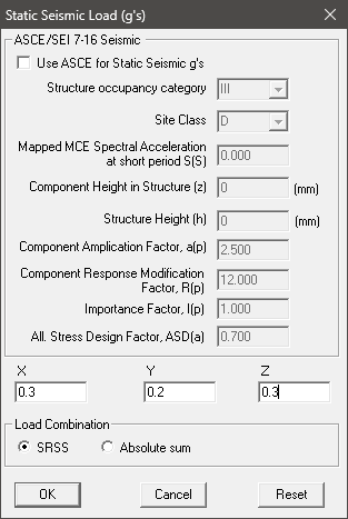
11. Static Seismic g’s: X=0.3, Y=0.2 and Z=0.3

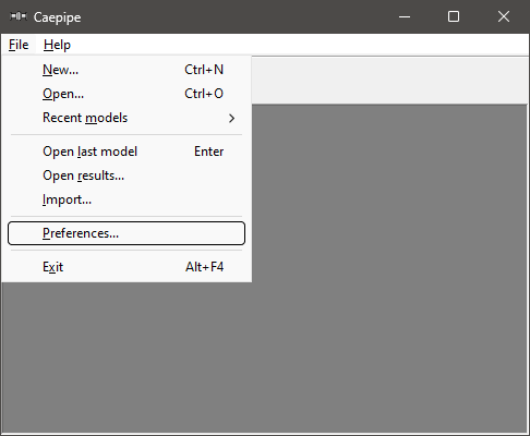
Start CAEPIPE. From the “File” pull down menu select “Preferences”.

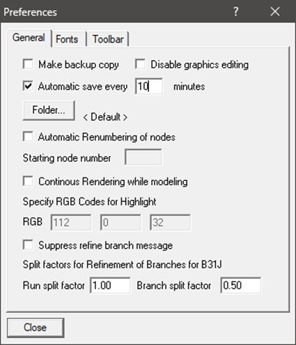
Make sure that the “Automatic save feature” is enabled and the “Automatic Renumbering of nodes” feature is disabled.

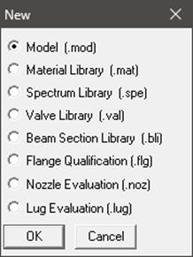
Start CAEPIPE. Then click on the “New” file button.

From the “New” ﬁle dialog, select the type of the new ﬁle as “Model (.mod)” ﬁle. This opens two independent windows: Layout and Graphics.

Layout window

Graphics window

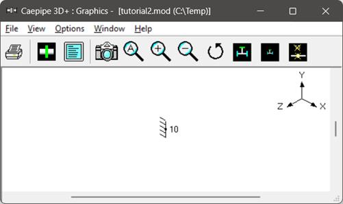
Adjust the size of the windows to ﬁt your desktop such that you can view both comfortably at the same time.

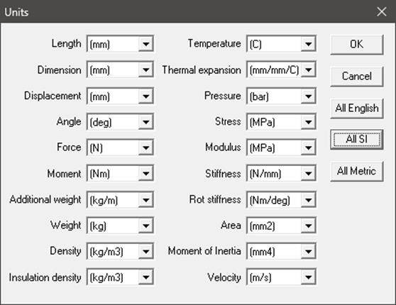
Change Units

As this is a SI/Metric model, change the units appropriately. From the layout window, click on “Options menu > Units” (alternately, press the hotkey “Ctrl+U”). Click on “All SI” button followed by “OK”. The layout window will show the offsets (DX/DY/DZ) in mm units.

1. Enter Title

Type “Sample Problem 2” as the title in the ﬁrst row that contains “Title =”. Press Enter.

2. Select Analysis options (piping code etc.)

Click on the “Options” menu and then select “Analysis” (Options > Analysis) to specify options for analysis.

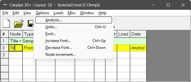
This opens the “Analysis Options” dialog.

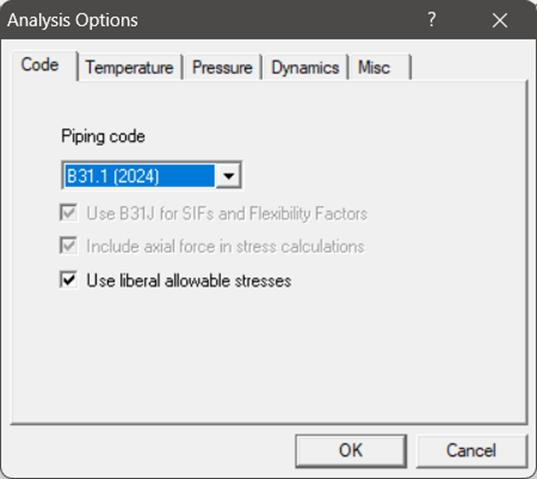
On the Code property page, select “B31.1 (2024)” for “Piping code”. Turn ON the option “Use liberal allowable stresses”. Then click on OK to close “Analysis Options” dialog.

3. Deﬁne Material, Sections and Loads

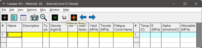
Click on “Matl” in the header in the Layout window (or press “Ctrl+Shift+M”)

This opens up the “Materials” list in a separate List window. Position and resize the list window as you desire. Click on “Library” button on the Toolbar (or “choose File > Library”).

The Open Material Library dialog is shown. If you don’t see the folder shown below, then navigate to the Material Library folder under the CAEPIPE installed folder (usually C:\CAEPIPIE3D\xxxx, xxxx = version number).

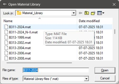
Select “B311-2024.mat” as the library file by double clicking on it. The available materials in the library are shown. Scroll down to “A312 TP 316”. Double click on it or click on “OK” to select it.

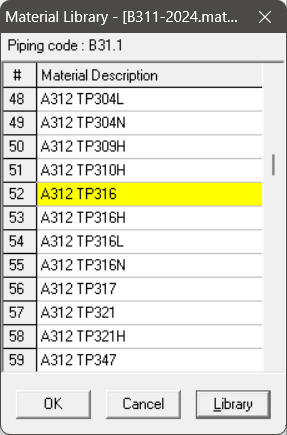
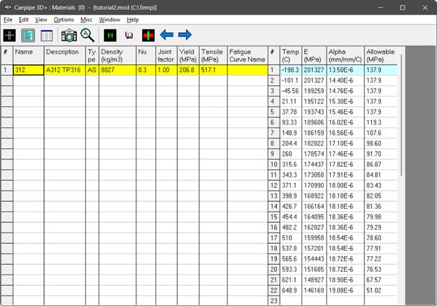
The properties for this selected material are transferred to the material in the List window. Type “312” for material name and then press “Enter”.

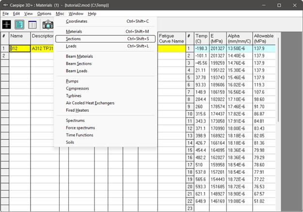
Sections

Select “Sections” from the “Misc” menu of the List window (or press “Ctrl+Shift+S”).

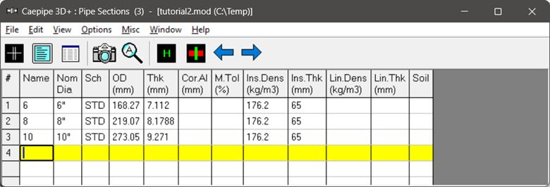
A list of Sections is shown. This system has three sections: 6”, 8” and 10”. To enter the ﬁrst section, type ‘6’ for “Section name” and press “Enter”. The “Section #1” properties dialog is shown with the section name 6.

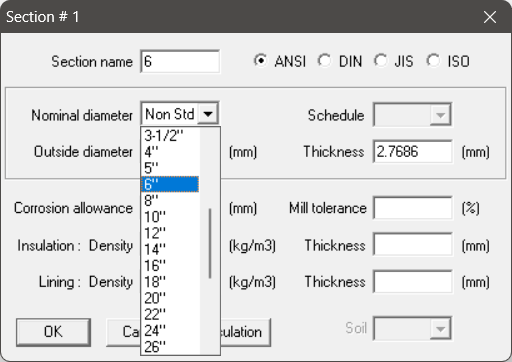
Click on the down arrow of the dropdown combo box for “Nominal diameter” and select 6” for “Nominal diameter”. Select/Enter other properties (STD thickness, Insulation density [Alt+I] may be used for a list of insulation materials or you may enter your own density, in this case, 176.2 kg/cu.m] and thickness 65 mm).

After entering all properties, press “Enter” or click on “OK” to enter the ﬁrst section.

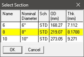
Now repeat the process for the 8” pipe section.

In row # 2, Type 8 for “Section name” and press “Enter”. The “Section Properties” dialog is shown with the section name 8. Select 8” for “Nominal diameter”, STD for “Schedule”, and same insulation properties as before for “Insulation”. Press “Enter” or click on “OK’ to enter the second section. Do similarly for the 10” pipe section.

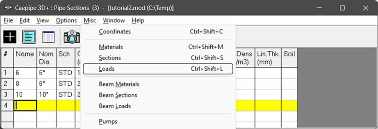
Load

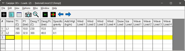
Select “Loads” from the “Misc” menu (or press “Ctrl+Shift+L”).

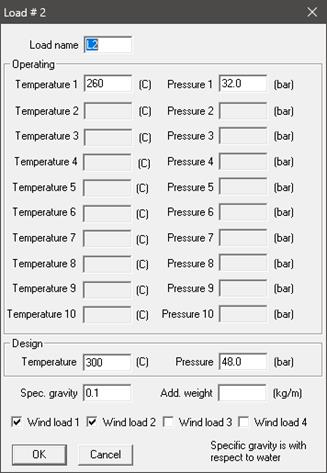
The Loads list is shown. To enter the ﬁrst load, Type ‘L1’ for “Name”, Tab to “T1” and type 185, Tab to “P1” and type 10 bar, tab to “Desg.T” and type 230, Tab to “Desg.Pr.” and type 15 and Tab to “Speciﬁc gravity” and type 0.1. Then press “Enter”. That is it! The load is entered. (Alternately, you could have pressed “Ctrl+E” on the ﬁrst row and typed in the same information in a dialog box). Similarly, enter the second load set “L2” {260°C, 32 bar, 300°C, 48 bar and Sp. Gravity = 0.1}.

Click in the “Layout window” or press “F3” to move the focus to the “Layout window’.

4. Input Model Layout

We are going to model the 10” main line ﬁrst, followed by the 8” segment.

CONVENTIONS

· In the following text, the word ‘type’ should be distinguished from the words ‘Type column’ or simply ‘Type’ (upper case ‘T’). The former (‘type’) will mean press the keys on the keyboard. The latter word ‘Type’ will refer to the “Type column” in the Layout spreadsheet. Of course, occurrence of Type at the beginning of a sentence will mean type the keys.

· Also, the instruction “type B for Bend” does not necessarily mean the upper case ‘B’. The lower case ‘b’ can also be typed.

· For items in the “Data” column (such as “Anchor” or “Hanger”), the cursor needs to be in the “Data” column. To move the cursor quickly to that column, press “Ctrl+Shift+D” from any column or click in the “Data” column. Or press the Tab key repeatedly to reach the “Data” column.

· As the graphics window is simultaneously updated, you should position the graphics window in such a way that you can see it along with the input window. Simultaneous feedback is one of the chief design intents in CAEPIPE.

· For mouse clicks, when you read the word “click on xxx,” this means left-click on your mouse. For the context menu, if referred to, right-click.

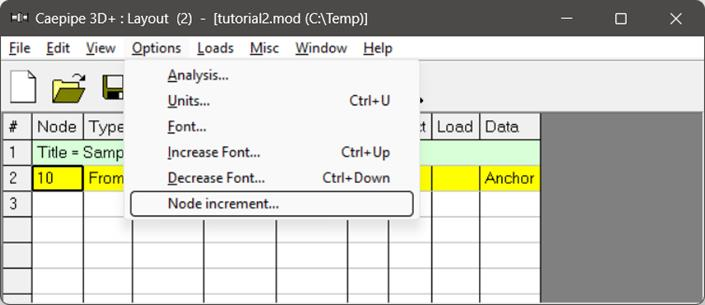
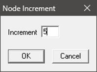
Change Node Increment

You might have noticed in the model drawing that the node numbering scheme has an increment of 5. CAEPIPE has a feature that allows you to specify a node increment. Select “Options menu > Node increment”…type 5 for value. Click on “OK”.

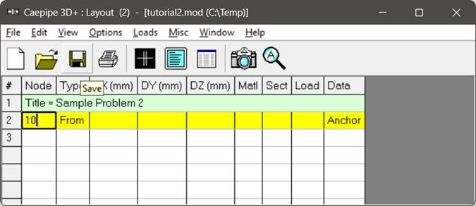
After defining the above parameters,

Save the model by clicking on the Save button.

The “Save Model As” dialog is shown.

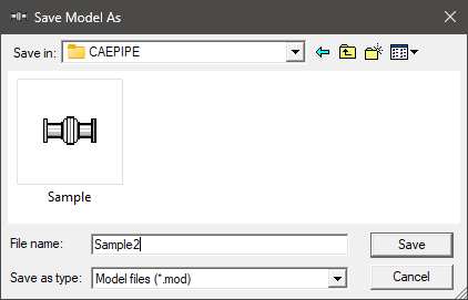
Type the File name as “Sample2” and press “Enter” to save the model.

First model the 10” Main line

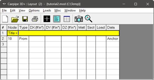
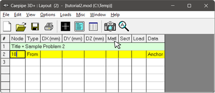
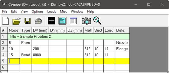
Following the “Title” at row #1, row #2 is already generated with Node 10 of Type “From” with an Anchor in the “Data” column.

Model information shows that the piping is connecting to a Nozzle of a Cylindrical Vessel with node number as 5. So, to account for the stiffness of the Nozzle protruding out of the Cylindrical Vessel, the nozzle portion is modeled as a pipe in this model. The junction of this Pipe (Nozzle) and the Shell is modeled as “Nozzle”.

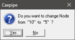
To change the Node number and to replace “Anchor” with “Nozzle”, click on 10, press Backspace to erase 10, type 5. Press Tab to advance. Confirm the node number change when asked (by clicking on Yes, or simply pressing the Spacebar key on the keyboard).

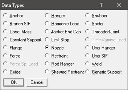
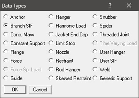
To replace the “Anchor” with “Nozzle”, highlight the data type “Anchor” at row #2 using mouse left button and then click on “Data” in the header in the Layout window. From the “Data types” dialog box shown, select the new data type as “Nozzle”.

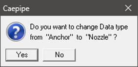
CAEPIPE will prompt as shown below. Press “Yes” to proceed.

Enter the Nozzle and Vessel parameters as shown below and press “OK”.

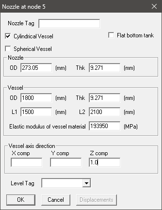
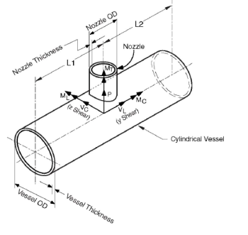
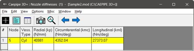
From the snap shots shown above, Lengths L1 and L2 on either side of the nozzle are the distances from the nozzle center line to the nearest location on vessel where the "ovalization deformation" of the vessel is stopped such as at a stiffener on the inner or outer surface of the vessel, or at the center of a saddle support to the vessel or at the junction to the torispherical enclosure (also called the head) or at a tube sheet inside the vessel etc. Nozzle stiffness computed by CAEPIPE can be seen through Layout window > View > List > Nozzle Stiffnesses.

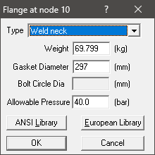
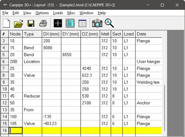
Now, press Enter to move the highlight to the next row (#3). Tab to the Type column. The next Node 10 is automatically assigned. Tab over to DX, type 200 (mm), Tab over to Material, press Enter to open the list of materials and select 312. Next Tab over to Section and press Enter. Select section 10 and press OK. Tab over to Load and press Enter, select L1 and click OK. Tab again to Data to input the flanges mating with the pipe and the equipment nozzle. Type “fl” to model flange and enter the data as shown below and press OK. CAEPIPE moves the highlight automatically to the next (new) row (#4).

Tab to the type column. The next node 15 is automatically assigned. Node 15 has a LR (long radius) bend (in CAEPIPE, a bend node is defined always at the tangent intersection point, being such, this node does not exist on the physical bend). Tab to the Type column; type “ben” to insert a default LR bend. Tab to DX, type in 8080 (mm), press Enter. CAEPIPE automatically enters the material, section and load from the previous row and moves the highlight to the next new row.

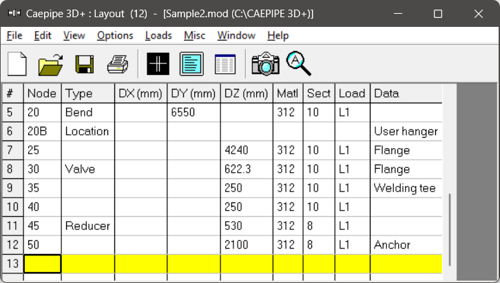
The following vertical bend (at node 20) can be modeled as before. Tab to Type (node 20 is automatically inserted), and type “ben” to insert a default LR bend, Tab again to DY, type 6550 (mm) and press Enter.

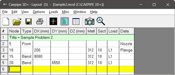
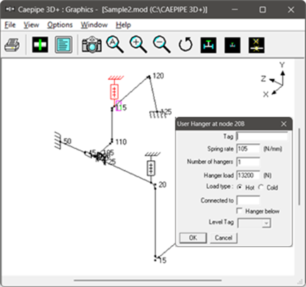
This bend has an already existing hanger (called “User Hanger” in CAEPIPE) at the far end, referred to as node 20B, an internally generated bend node.

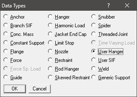
So, on the next row, type 20B for Node, Tab to Type, press “L” for Location, which spawns the available data types you can insert at this node. Pick “User Hanger” from the dialog.

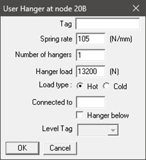
Enter its properties as shown. Click on OK.

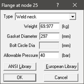
Next, the line moves in the Z direction to the flange node 25. Pressing Tab on the new row generates node 25 for you. Tab to DZ, type 4240, (click in Data column) or press Ctrl+Shift+D to move cursor to Data column. Type “fl” to open the Flange Data type dialog. Enter the details shown below and press OK.

A valve is placed next from Node 25 to Node 30, where another mating flange is located. Pressing Tab on the new row generates node 30. Tab to the Type column; type “v” to insert a “Valve” and enter the data as shown below and press OK.

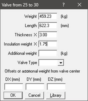
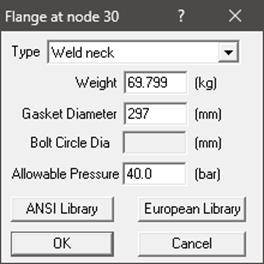
Tab to Data and type “fl” to enter a “flange”. Type “fl” to open the Flange Data type dialog. Enter the details shown below and press OK.

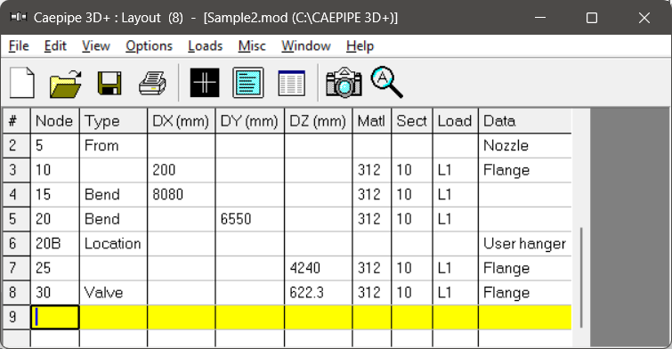
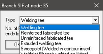
Next model a pipe element till node 35 (welding tee). Press Tab for node 35, Tab to DZ, type 250, (click in Data column) or press Ctrl+Shift+D to move cursor to Data column. Type “br” (or right-click in Data, select Branch SIF) to open the Tee types Data type dialog. Select Welding Tee from the dropdown box. Click on OK (or press Enter).

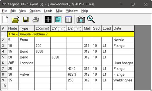
Next model a pipe element till node 40. Press Tab for node 40, Tab to DZ, type 250 and press Enter.

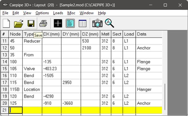
The next element is a 10x8 concentric reducer. Here is how to model it. Tab for the next node # (45), type “red” for Reducer in the Type column. CAEPIPE displays the Reducer dialog with the current section properties.

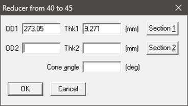
Click on “Section 2” button to select the following section, in this case, the 8” section. After placing the highlight on the 8” section, press Enter (or click on OK).

You are back at the Reducer dialog.

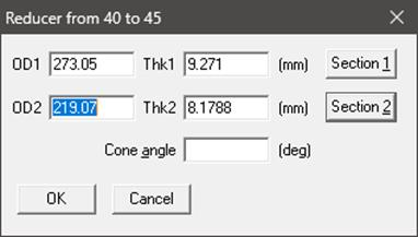
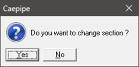
Click on OK to finish inserting the reducer. On the layout screen, type 530 for DZ and press Enter, at which point CAEPIPE wants you to confirm the section change. Click on Yes.

Then select 8 as the new section from here on. Press Enter to move to next row.

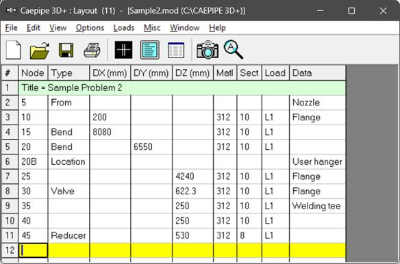
The last element here is an 8” pipe that ends at node 50. As before, press Tab for Node 50, type 2100 for length in the same direction. Press Ctrl+Shift+D to go to Data and press A to insert a rigid anchor (note that CAEPIPE inserts the correct old material, new section and old load for this row).

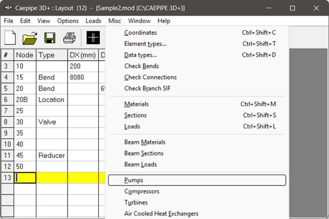
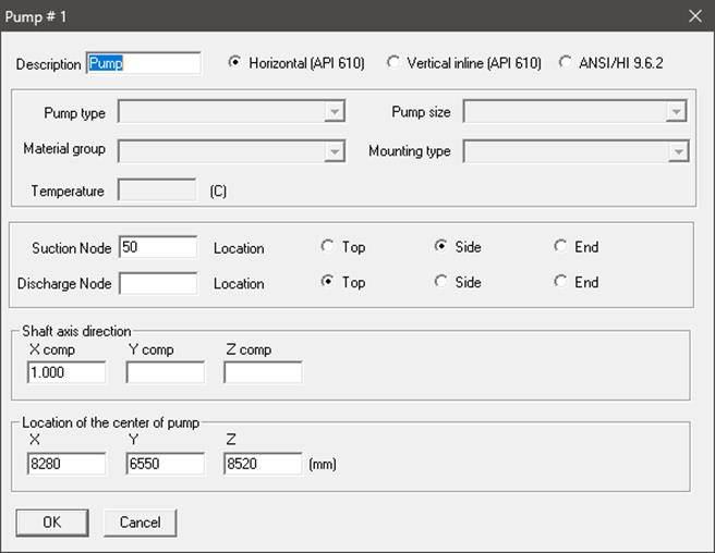
Click on the Zoom All button (or press Ctrl+A) to view the header line fully in the graphics window.

Node 50 is connecting to a Side Suction Nozzle of an API 610 Horizontal Pump. To model this, select the option “Pumps” through Layout Window > Misc. Double click on an empty row and enter the values as shown below. Once modeled, CAEPIPE will automatically perform the Pump Qualification and shows the report in Results.

Now the 6” branch

On the next row (#13), type 35 for Node, Tab to the Type column, type ‘f’ (for “From”, since we are beginning a new branch from an existing Node 35), press Enter. In the next row (#14), type “100” in the Node column to clearly identify the new branch. Tab to DX and enter –135. CAEPIPE inserts the previous material, and automatically detects the new branch and asks if you want to change section.

Since we want to change the section to 6, click on Yes. This opens the Section selection dialog.

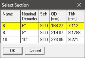
Select the 6” section by double clicking on it. The section (6) is entered in the Section column in the Layout window. The load is again automatically inserted from the previous load. Lastly, type “fl” in the Data column and hit enter to create a mating Flange. This will bring up the Flange type dialog box.

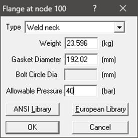
Type in 23.596 for Weight, 192.02 for Gasket Diameter, 40 for Allowable Pressure and click Ok.

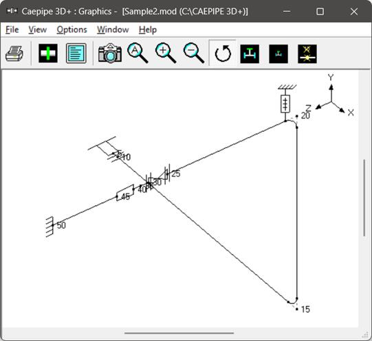
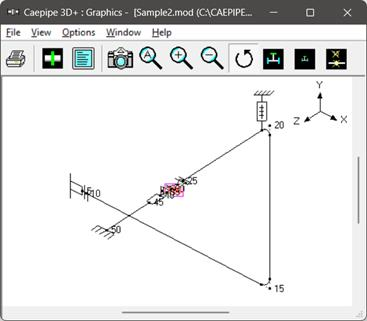
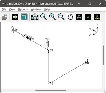
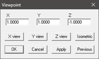
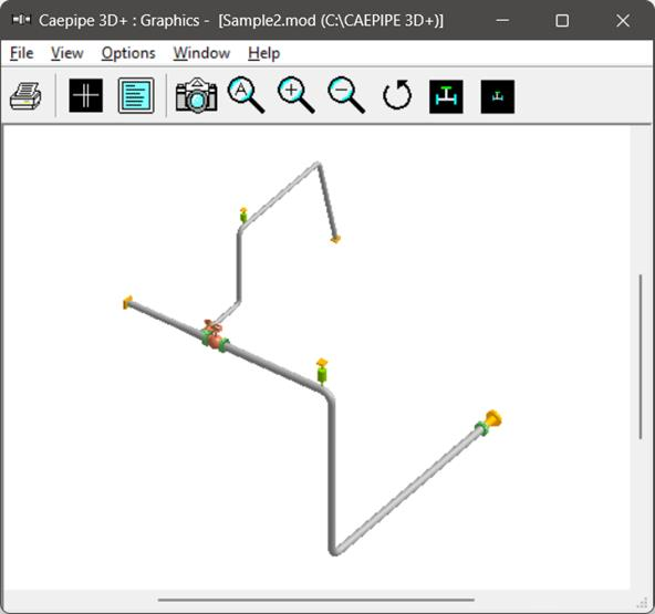
The graphics window will look like this. For better view, rotate the model by clicking the icon

and scrolling the horizontal scroll bar towards left using the mouse left button or through keyboard left arrow key. Alternatively, you can specify the viewpoint as shown below by selecting the icon

from the graphics frame.

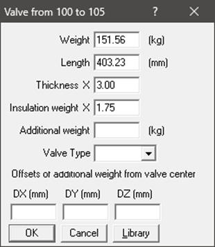
In the next row (#15), Tab to the Type column. The next Node 105 is automatically assigned. In the Type column, type ‘v’ (for Valve). This brings up the Valve dialog box. In the Valve dialog box, type 151.56 for Weight, 403.23 for Length, 3.00 for Thickness, and 1.75 for Insulation weight. Then press Enter or click on OK to input the valve. Press Enter again.

You will see that the DX, Material, Section and Load information is automatically input in the Layout window.

You can now copy the flange along with data from Node 100 and paste it at Node 105. To perform this, highlight row # 14 and press Ctrl+C. Then move the cursor to Data column of row #15 and press Ctrl+V to paste the flange. Press Enter to move to the next row.

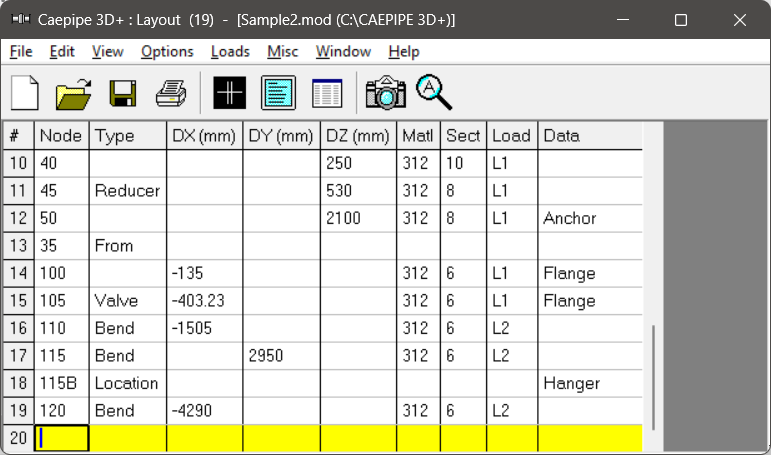
In the next row (#16), Tab to the Type column, type “ben” to create a Long Radius Bend and then Tab to the DX column. The default LR Bend is automatically input when you Tab over. In the DX column type –1505 and hit Enter. The Material, Section and Load information and is automatically input. As the Temperature and Pressure is changing from this element, change the Load from L1 to L2 by right clicking on the “L1” in the Load field.

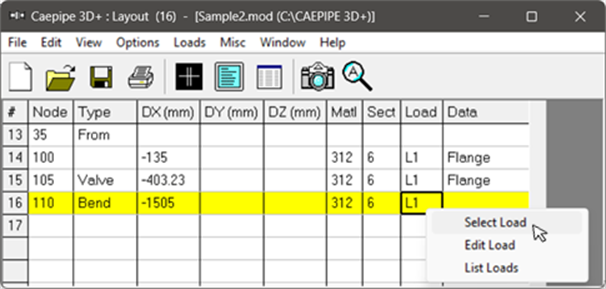
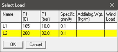
This will bring up a small Context menu from which you will choose Select Load. This will bring “Select Load” window. Highlight L2 and click Ok. Press Enter to complete inputting Node 110 at row (#16).

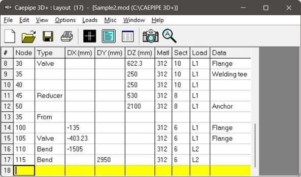
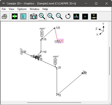
In the next row (#17), create another Long Radius Bend just like the one in row (#17), except change the DX -1505 to DY 2950 and press Enter. Your layout window should look like this.

Start the next row (#18) by typing 115B in the Node column. Tab to the Type column and type “L” to specify a Location type. This will automatically open the Data Types dialog box. Select Hanger.

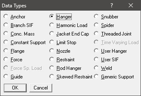
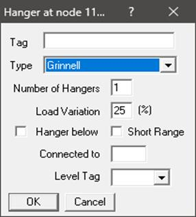
Another dialog box will appear with specific Hanger type input options. Keep the default settings and click OK.

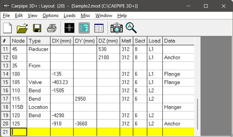
At Node 120 on the next row (#19), Tab to the Type column and input a default LR Bend by typing “ben”. Tab to the DX column and input –4290 and press Enter.

On the next row (#20), Tab over to the DX column and input -910, then in DY input –3660. Create an Anchor in the Data column by either pressing Ctrl+Shift+D or Tabbing to the Data column and typing “a”. Press Enter and you are done with Layout window input.

Define “Static seismic” through Layout Window > Loads > Static Seismic 1. Enter the value as shown below.

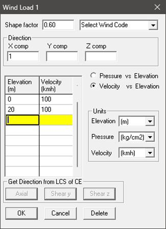
Let us define “Wind Load” profile in +X direction through Layout Window > Loads > Wind 1 and enter the data as shown below and press OK. The maximum elevation of 20m is chosen so that the entire piping system experiences wind load.

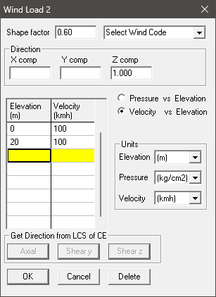
Similarly, define “Wind Load” profile in +Z direction through Layout Window > Loads > Wind 2 and enter the data as shown below and press OK.

Assign the Wind Load defined above to the stress layout through Layout window > Misc > Loads and then double click on the Loads “L1” and select the check box “Wind load 1” and “Wind load 2” as shown below.

Similarly, select the check boxes “Wind load 1” and “Wind load 2” for “L2”.

5. Select Load Cases for Analysis

Select Loads cases from the Loads menu.

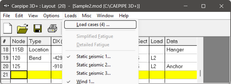
The Load cases dialog is shown.

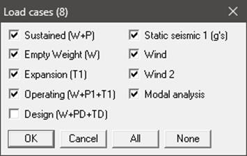
By default, Sustained (W+P), Empty Weight (W), Expansion (T1) and Operating (W+P1+T1) load cases are already selected. Add Static Seismic (g’s), Wind, Wind 2, and the Modal analysis Load cases by clicking on the checkbox next to it. Design (W+PD+TD) load cases when selected for the Analysis, CAEPIPE will compute and show results for Displacements, Element Forces & Moments, Support Loads and Support Load Summary. Design load cases do not include Stress Calculations, Rotating Equipment Qualifications and Flange Equivalent Pressure Calculations. Press OK to return to the Layout window. The model input is now complete.

Click on the Zoom All button (or press Ctrl+A) to show the whole model in the graphics window.

To see a 3D rendered view of the model, click on the Render button (or press Ctrl+R) in the graphics window.

To return to the non-rendered view, click on the Do not render button (or press Ctrl+R).

List

One of the useful features of CAEPIPE is the ability to show a list of all like items such as anchors, bends etc. in a separate List window. Click on the List button (or press Ctrl+L) to show the list dialog.

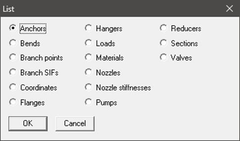
Click on an item of interest to show the list for that item.

A list of all the anchors present in this sample model is shown below:

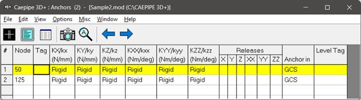
The highlighted item can be edited directly in the List window (in most cases) or in a dialog by pressing Ctrl+E. The items can be deleted by pressing Ctrl+X. The item is also highlighted in the graphics window by ﬂashing and with a box around the node number.

A list of all the bends in the sample model is shown below:

Editing in the Graphics Window

Another useful feature is the ability to edit an item in the graphics window. When an item such as a Hanger is clicked in the graphics window, a dialog box for that item is opened, where it can be modiﬁed.

Save the model by clicking on the Save button.

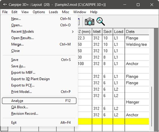
6. Analyze

Click on Analyze under the File menu.

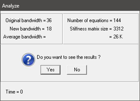
After the analysis, you are asked if you want to see the results. Select Yes.

7. View Results

After ﬁnishing the analysis and choosing to see the results or by opening the results ﬁle (.res), the results window is displayed. The Results dialog is opened automatically.

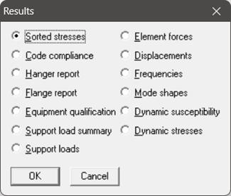
Select an item of interest by clicking on it. When you are viewing the results, use Tab (or Next Result button) to view the next result and Shift+Tab (or Previous Result button) to view the previous result. The Results dialog can be brought up by clicking on the Results icon (or press Ctrl+R).

While viewing the results, the model data can also be simultaneously viewed in separate Layout and List windows. These are now “read only” windows, i.e. the model data cannot be modiﬁed while viewing the results. Some of the results from the sample problem are shown below:

Sorted stresses

The computed stresses (sustained, expansion and occasional) are sorted in descending order by stress ratios.

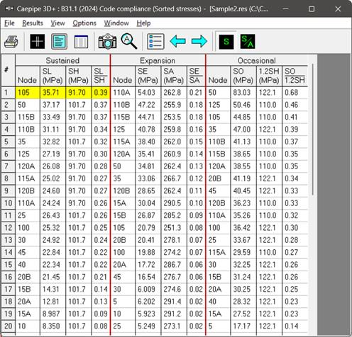
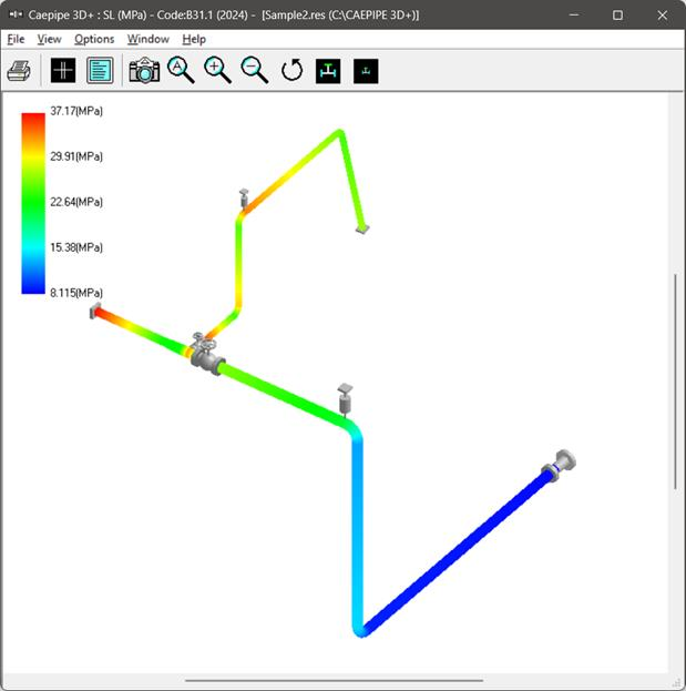
Color coded stresses may be rendered in the graphics window by pressing the Show stresses button (or choose View > Show Stresses). The stresses in the highlighted columns (the bar highlights three columns simultaneously) are displayed in the graphics window. Use the left and right arrow keys to change the highlighted columns or click in a particular column.

The stress ratios may similarly be rendered by using the Show stress ratios button (or choose View > Show Stress Ratios).

Instead of rendering color coded stresses/stress ratios, the values of stresses/stress ratios may be plotted by using the menu: View > No color coding and pressing the icon S or S/A.

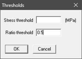
While plotting stresses or stress ratios, thresholds may be speciﬁed from the graphics window (choose View > Thresholds). Only those stresses or stress ratios exceeding the threshold are plotted.

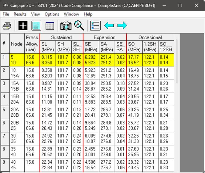
Code compliance

Element stresses and stress ratios calculated according to the selected piping code are shown under Code compliance. Design pressure and CAEPIPE computed Allowable pressure are shown in 2^nd column.

Hanger report

The hanger report is shown below.

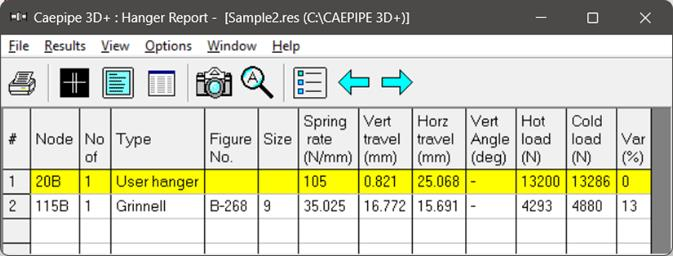
The “No of” ﬁeld shows the number of hangers required at the indicated location. The Figure No. and Size refer to the manufacturer’s catalog. The vertical travel (also referred to as “Hanger travel”) is the vertical deﬂection at the hanger location for the ﬁrst operating load case. Similarly, the horizontal travel is the resultant horizontal deﬂection at the hanger location for the ﬁrst operating case. The hot load is the hanger load for the operating condition and the cold load is the hanger load at zero deﬂection.

Variability (%) = (Spring rate × Hanger travel / Hot load) × 100

Flange report

The Flange report in the CAEPIPE results window shows the loads at each flange location for the operating case (W+P1+T1).

The Flange Pressure is an “equivalent pressure” calculated from the actual pressure in the piping element, the bending moment and the axial force on the flange for the first operating case (W+P1+T1)

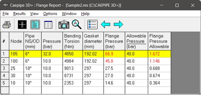
The last column shows a ratio of this “equivalent” Flange Pressure to a user-input Allowable Pressure. This ratio is flagged in red when it exceeds 1.0.

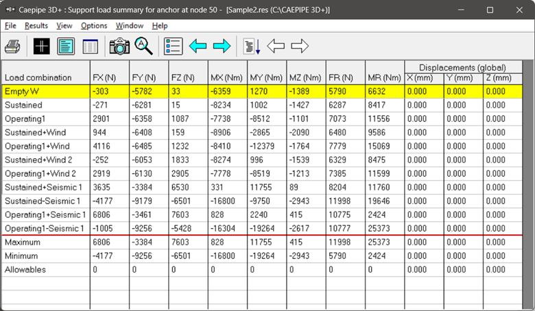
Support load summary

Support load summary for each support is created by considering all the load cases and appropriate combinations and then showing the maximum and minimum loads.

Note: Allowable loads at an equipment nozzle can be calculated using the module “Nozzle Evaluation” available in CAEPIPE through Main Frame > New > Nozzle Evaluation.

The allowable loads thus calculated can then be entered as “User Allowables” in CAEPIPE Stress Model through Layout window > Misc. See the CAEPIPE tutorial titled “Tutorial on Qualification of Nozzles to Equipment using CAEPIPE” for more details.

Use the Other supports button (F6), Next support button (Ctrl+Right arrow) or Previous support button (Ctrl+Left arrow) to see loads on other supports (e.g. other anchors, hangers etc.).

Support loads

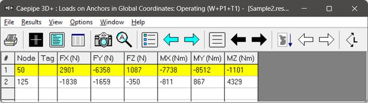
Support loads are the loads acting on all the supports of each support type for a specific loading case. The loads on anchors for the Operating load case are shown below.

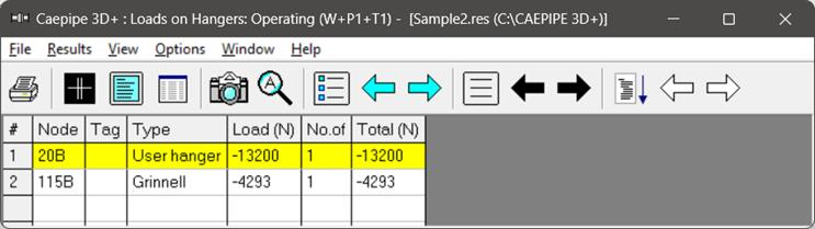
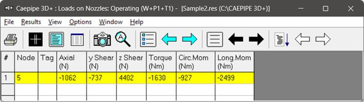
Use the Load cases button, Next load case button (Right arrow) or Previous load case button (Left arrow) to see loads for different load cases (e.g. Sustained, Expansion etc.).

Use the Other supports button (F6), Next support button (Ctrl+Right arrow) or Previous support button (Ctrl+Left arrow) to see loads on supports of different types (e.g. other anchors, hangers etc.).

The loads on hangers (i.e. the loads acting at the hanger locations imposed by the piping system) and the loads on the nozzle for the Operating case are shown below.

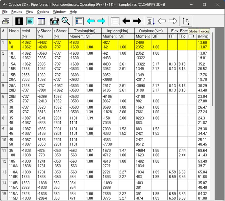
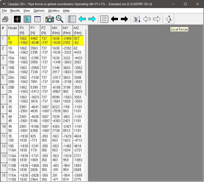
Element forces

For pipe (also bend and reducer), element forces in local coordinates, Stress Intensiﬁcation Factors (SIF) and stresses are shown by default for the selected load case.

Use the Local forces button (F7) to see the element forces in local coordinates again.

Use the Global forces button (F7) to see the element forces in global coordinates.

Use the Other forces button (F6), Next force button (Ctrl+Right arrow) or Previous force button (Ctrl+Left arrow) to see other element forces (e.g. valves, bellows etc.).

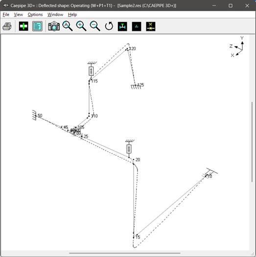
Displacements

The nodal displacements are shown.

Use the Load cases button, Next load case button (Right arrow) or Previous load case button (Left arrow) to see loads for different load cases(e.g. Sustained, Expansion etc.).

Use the Deﬂected shape button (or View > Show deﬂected shape) to plot the deﬂected shape in the graphics window.

Use the Animated deﬂected shape button (or View > Show animated deﬂected shape) to plot the animated deﬂected shape in the graphics window.

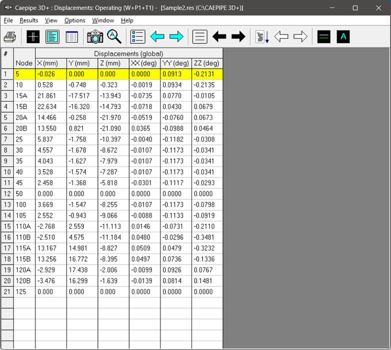
Choose View > Magniﬁcation to change the magniﬁcation of the deﬂected shape.

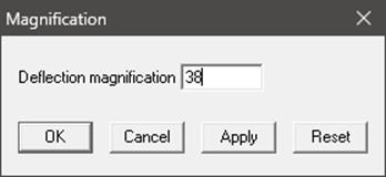
The reset button is used to calculate a default magniﬁcation factor which scales the maximum deﬂection to about 5% of the width of the graphics window.

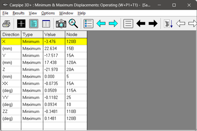
Use the Other displacements button (F6), Next displacement button (Ctrl+Right arrow) or Previous displacement button (Ctrl+Left arrow) to see other displacements (e.g. Min/Max, displacements at hangers, ﬂex joints, limit stops etc.).

The minimum and maximum displacements for each of the directions and the corresponding nodes are shown below.

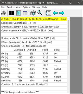
The Pump qualification report (Rotating Equipment report) is shown below.

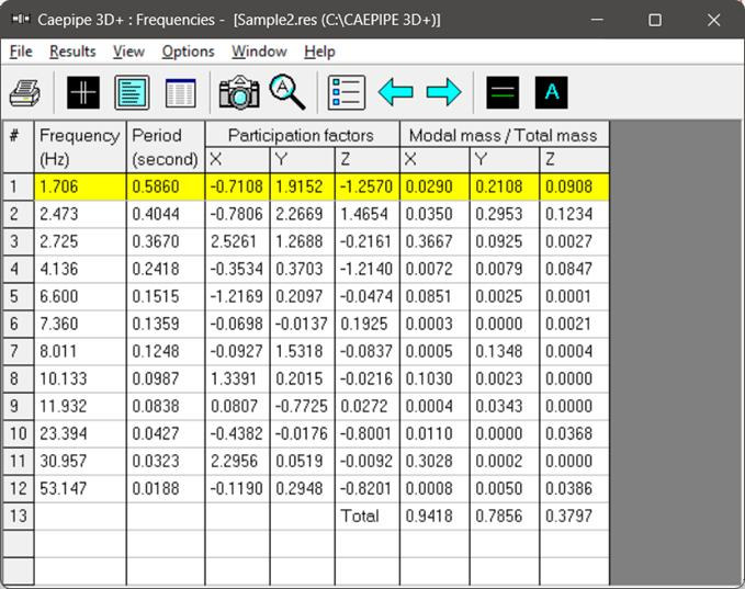
Frequencies and Mode shapes

A list of natural frequencies, periods, modal participation factors and modal mass fractions is shown next. You can show each frequency’s mode shape graphically or animate it by clicking on Show mode shape or Show animated mode shape button in the toolbar.

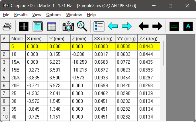
Each frequency’s mode shape detail is shown in the next window. As in the earlier window, you can show graphically the mode shape or animate it by clicking on the appropriate button.

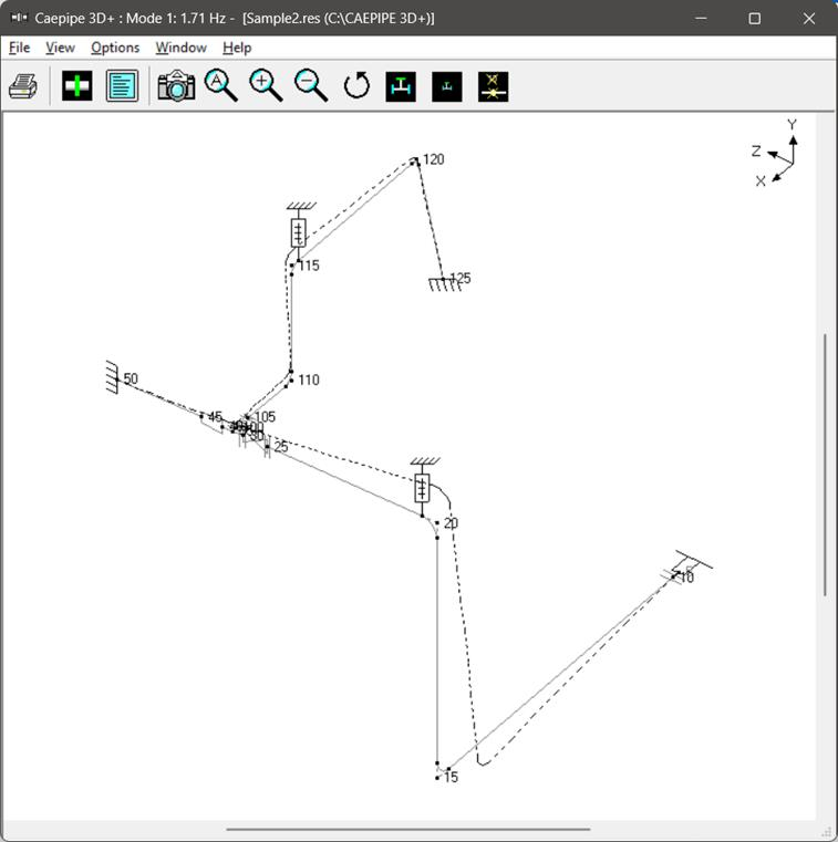
The graphic window will show the mode shape as below.

Use the black arrow buttons to cycle through the different Modes.

Dynamic Susceptibility

Note: Dynamic Susceptibility is NOT available for Evaluation Version of CAEPIPE. For Full Version of CAEPIPE, this feature can be turned ON by setting an environment variable “HARTLEN” that needs to be declared under My Computer or This PC Icon > Mouse Right Click > Properties > Advanced System Settings > Environmental Variable with its Value set to (YES). Refer to CAEPIPE User’s Manual for more details.

The stress / velocity method, implemented in CAEPIPE as the “Dynamic Susceptibility” feature, provides quantified insights into the stress versus vibration characteristics of the system layout per se.

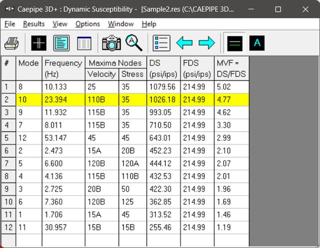
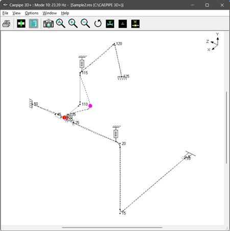
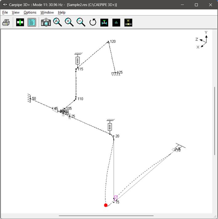
Pressing the Animated mode shape button (or View > Show animated mode shape) for Mode 10, for example, shows the maximum dynamic bending stress at the Bend Node 35 (RED dot) and the maximum velocity at the Bend Node 110B (PINK dot).

In case the maximum dynamic bending stress and the maximum velocity occur at the same node for a specific mode, then the RED and PINK dots overlap with each other and only the RED dot is seen for that mode. See the Animated mode shape shown below for mode 11 as an example.

The dynamic susceptibility module does not apply directly to meeting code or other formal stress analysis requirements. However, it is an incisive analytical tool to help the designer understand the stress / vibration relationship, assess the situation and to decide how to modify the design if necessary to possibly reduce the susceptibility to vibration. It can be used for design, planning acceptance tests, troubleshooting and correction.

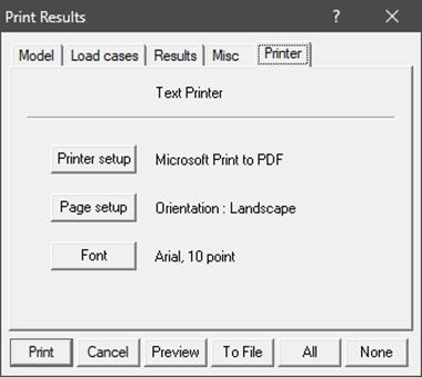
Print

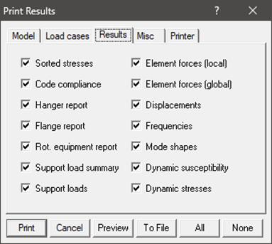
To print results and model data, click on the Print button (or press Ctrl+P). In the Print Results dialog, the items to print can be selected.

You can also print to a text ﬁle by using the To File button. A preview of the printed output can be seen by using the Preview button.

The printing options such as choice of printer, margins, portrait or landscape and font can be set on the Printer tab.

The sample problem report is shown next. Note that for sorted stresses and code compliance, wherever the stress ratio exceeds 1.00, the corresponding stress and stress ratio are shown in white letters on black background. Similarly, wherever the Flange Pressure exceeds the Allowable Pressure, the corresponding Flange Pressure and the ratio are shown in white letters on black background.

This is the end of the tutorial. If you have questions or comments, please email them to: support@sstusa.com