Tutorial on Wave Loading Analysis by CAEPIPE

Introduction

Wave loading refers to the dynamic forces exerted by ocean waves on offshore and coastal structures, including piping systems. In piping stress analysis, particularly for marine pipelines, risers, or platform-mounted piping, wave loading is a critical consideration due to its potential to induce significant dynamic stresses, vibrations, and fatigue over time. In most piping stress analysis software including CAEPIPE, Wave Loading is included as Static Equivalent Force, ie., the maximum force that waves apply on a given component.

When waves interact with submerged or partially submerged pipes, they generate forces primarily due to:

· Drag Forces – caused by the relative motion of the water past the pipe.

· Inertia Forces – resulting from the acceleration of the surrounding water mass.

· Lift Forces – generated due to asymmetry in flow (especially if currents are present).

· Buoyancy Forces – due to the weight of displaced fluid.

To quantify these forces, the Morison Equation is widely used. It provides a semi-empirical method for calculating wave-induced forces on slender members (like pipelines), combining drag and inertia effects. The Morison's equation gives distributed wave force (drag + inertial) per unit length of the member and is normal (perpendicular) to the member. It is written as,

where,

Cd = Drag Constant =

Cm = Inertia Constant =

CD = Drag Coefficient. See Note below.

CM = Inertia Coefficient. See Note below.

= Density of Sea water

D = Outer Diameter of Pipe / Pipe Components inclusive of Insulation Thickness and Marine Growth Thickness.

u = Fluid particle velocity

= Fluid particle acceleration

f = Drag and Inertia Force acting on the pipe element per unit length.

Key Parameters influencing Wave Loading:

· Wave height and period (determining wave energy)

· Submergence depth of the pipe

· Pipe orientation and support conditions

· Presence of currents (which modify particle velocities)

· Marine growth (increasing effective diameter and drag)

Wave Parameter Inputs

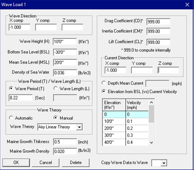
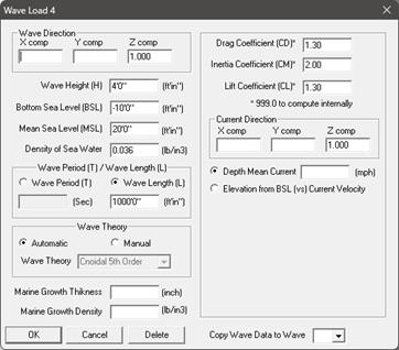
Wave Direction

Input the direction of the wave using the direction cosines (for example: When the vertical axis is parallel to Global Y, for wave in Z direction, X comp = 0.0, Y comp = 0.0, Z comp = 1.0; for wave in 45° X-Z plane, X comp=0.707, Y comp=0.0, Z comp=0.707). See section titled “Direction” in this CAEPIPE User’s Manual. CAEPIPE will allow inputting the wave direction only in the horizontal plane and NOT in the vertical direction.

Mean Sea Level and Bottom Sea Level

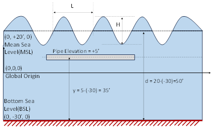
Mean Sea Level (MSL) is the distance of the mean water surface from the global origin (it could be positive or negative). It is NOT a measure of the depth of the pipe’s centerline.

In the 1^st figure below, the distance of the water surface is 20’ feet above the global origin. The horizontal pipe starts at, say, (10, 5, 0). So, the pipe is submerged 15’ (= 20’ - 5’) below the Mean Sea Level into the water.

Similarly, Bottom Sea Level (BSL) is the distance of the sea bed level from the global origin (it could be positive or negative). In the 1^st figure below, the distance of the sea bed is -30’ feet below the global origin. So, the pipe is located at a distance of 35’ feet from the Bottom Sea Level. This is indicated as “y” (pipe centreline from BSL) in the figure.

Wave Depth (d) is computed as the difference between the Mean Sea Level and Bottom Sea level (i.e., d = MSL – BSL). So, in the 1^st figure below, d = 20 – (-30) = 50’0”.

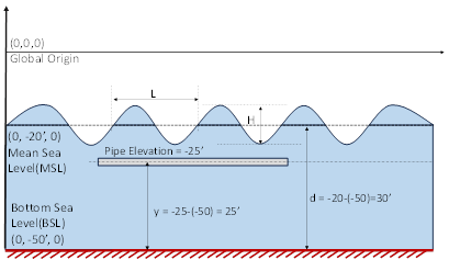
Given below is another example, wherein the global origin is above the Mean Sea Level (MSL).

Density of Sea Water

Input the density of Sea Water. Seawater density varies depending on temperature, salinity, and pressure. The average density of ocean is about 1030 kg/m³.

Wave Period / Wave Length

Input one of the following: wave period (sec) or wave length (ft or mm). Depending upon the Wave Theory selected, CAEPIPE will internally compute the other parameters using the dispersion relation. For example, if you input the wave period, CAEPIPE will automatically calculate the wavelength (or vice versa) based on the selected wave theory (either chosen manually or determined automatically when the 'Wave Theory' option is set to 'Automatic').

Wave Theories

The following wave theories are available for manual selection or will be automatically chosen by the program when the 'Wave Theory' option is set to 'Automatic'.

1. Airy’s Linear Theory

2. Stokes 5^th Order

3. Cnoidal 5^th Order

Airy’s Linear Theory

The Airy’s linear wave theory is the simplest and most useful theory among various wave theories. It assumes small wave steepness (H/L) and small relative water depth (H/d), which allows the free surface boundary conditions to be linearized and satisfied at the Mean Sea Level (also known as Still Water Level, SWL).

Stokes 5th Order

The Stokes wave theory assumes that the velocity potential and free water surface level as power series in terms of a non-dimensional small perturbation parameter

which is defined as the product of wave number and wave amplitude. Stokes 5^th Order theory considers power series until 5^th order. Stokes wave theory is most useful when the depth to wave length ratio, d/L is greater than 1/8 to 1/10.

Cnoidal 5th Order

Finite amplitude long waves of permanent form in shallow water are better described by the Cnoidal wave theory. The Cnoidal wave is a periodic wave that usually has sharp crests separated by wide troughs. The theory accounts for a large class of long waves of finite amplitude. The approximate range of validity of the theory is d/L < 1/8 and the Ursell parameter,

. Note that the Ursell parameter is defined as UR = HL²/d³.

To apply any of the theories listed above, enter the required parameters for the wave. CAEPIPE uses these parameters along with the dispersion relation to determine the wave length or wave period.

After calculating the wave length (L) and/or wave period (T), CAEPIPE determines the horizontal and vertical particle velocities (u & v), as well as the horizontal and vertical particle accelerations (du/dt & dv/dt), for various phase angles at 22.5 degree intervals (from 0 to 180 degrees) at the pipe centerline elevation, referenced from the bottom sea level. These velocity and acceleration values at each phase angle are then used in Morison’s equation (in both horizontal and vertical directions) to compute the maximum concentrated forces due to Drag, Inertia and Lift in the three global directions (FX, FY and FZ) at each node.

Wave Theory Selection

User can select the Wave Theory Manually or instruct CAEPIPE to determine the appropriate Wave Theory by selecting the option “Automatic”.

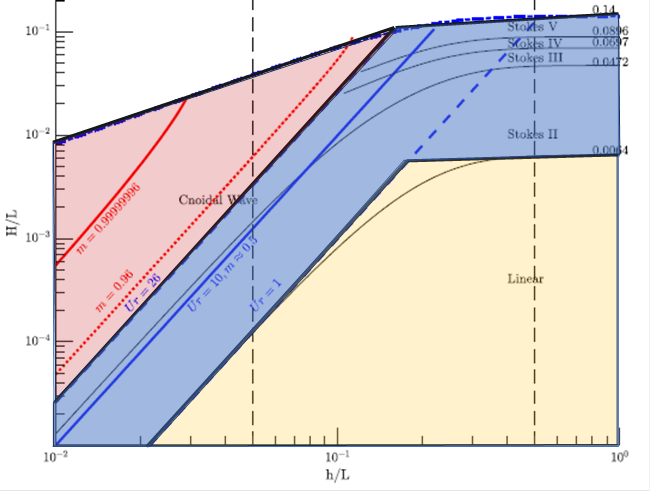
When the option “Automatic” is selected, then CAEPIPE computes the Ursell (UR) parameter using the wave parameters input in the dialog along with the chart given below to decide the Wave Theory. Ursell parameter is defined as UR = HL²/d³, where d = Wave Depth as explained above, H = Wave Height and L = Wave Length.

“Airy’s Linear Theory” is selected when UR < 1.00 and H/L < 0.0064. This region is shown in YELLOW in the below chart.

“Stokes 5^th Order” is selected when the UR computed internally is within the BLUE region shown below in the chart, and

“Cnoidal 5^th Order” is selected when the UR > 26.0 and within the RED region shown below in the chart.

Note:

If Wave Length required for computing the Ursell parameter is not input, then CAEPIPE computes the Wave Length by solving the dispersion relation as per Airy’s Theory using Wave Period.

Marine Growth Thickness and Density

The effect of accumulation of algae, sea weed, coral, etc., surrounding the pipe can be considered in the analysis by specifying the Marine Growth Thickness and Density. Marine Growth leads to an increase in Outer Diameter of the piping thereby affecting the Buoyancy, Weight of the piping and Wave Kinematics. In addition, when you input a non-zero value for Marine Growth Thickness in the dialog, then CAEPIPE considers the pipe surface as “Rough” while determining the Drag, Inertia and Lift coefficients. On the other hand, when the Marine Growth thickness is input as 0.00 or left BLANK, then CAEPIPE considers the pipe surface as “Smooth” while computing these coefficients.

Drag, Inertia and Lift Coefficients

The Drag Coefficient (CD) represents the resistance encountered by the body due to the flow of fluid (viscous effects). The Inertial Coefficient (CM) captures the accelerative impact of wave forces generated by the pressure field around the body. The Lift Coefficient (CL) indicates the normal force perpendicular to the flow, arising from phenomena like vortex shedding and asymmetric flow patterns.

Any of the coefficients can be entered in the following ways:

· Non-zero positive value: Applied to all elements selected for the wave analysis, considering both horizontal and vertical fluid velocities and accelerations.

· +999.0: CAEPIPE computes the corresponding coefficient internally and applies it to the elements selected, considering both horizontal and vertical fluid velocities and accelerations.

· Non-zero negative values: The absolute value of the coefficient entered will be used, but only horizontal fluid velocities and accelerations are considered (vertical components are excluded).

· -999.0: CAEPIPE computes the value internally and applies it to the elements selected, but only horizontal fluid velocities and accelerations are considered (vertical components are excluded).

· Zero (0.0): The effect of that force is ignored entirely in the analysis (e.g., setting CD to 0.0 ignores Drag force).

Wave Load Application in CAEPIPE

At present, in CAEPIPE V14.00, user can enter up to four (4) wave load data namely Wave Load 1, Wave Load 2, Wave Load 3 and Wave Load 4.

User can apply a wave load to the whole or parts of the model. To apply the wave load to the required portion of the layout, input "Y(es)" under the Layout Window > Misc > Loads > Wave Load 1/Wave Load 2/Wave Load 3/Wave Load 4. When done, CAEPIPE internally computes wave load for each element and applies the corresponding forces and moments equally at the two nodes of each element.

When an element is subjected to a wave load, CAEPIPE computes forces due to Drag, Inertia and Lift due to Horizontal particle Velocity, Current Velocity and Horizontal particle Acceleration as well as Drag, Inertia and Lift due to Vertical particle Velocity and Vertical particle Acceleration. The forces thus computed are considered in Occasional load case.

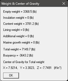
Apart from the above, the element is also subjected to Buoyancy force. At present, this buoyancy force is computed using the properties input under Wave Load 1. This effect reduces the apparent weight of the piping as it acts against the gravity. Hence, the Buoyancy effect is included in Sustained load case.

Drag and Inertia forces generally act in the direction of the wave velocity and Lift force will be normal to the direction of the wave velocity. For example, when the wave direction is parallel to Global Z with Vertical axis being parallel to Global Y, then the Drag and Inertia forces will act in Global Z direction and Lift force will be in the plane normal to Global X and Z directions (i.e., parallel to Global Y direction). For further details, refer to the Section titled “Wave Load” in CAEPIPE Code Compliance Manual.

Below is a sample tutorial that has 4 waves with 3 manual selections (Airy’s, Stokes 5^th Order, Cnoidal 5^th Order) and 1 automatic selection of wave theory.

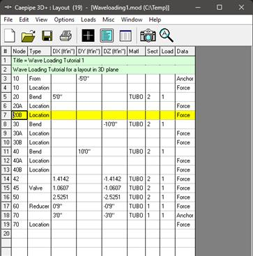
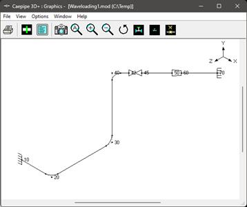
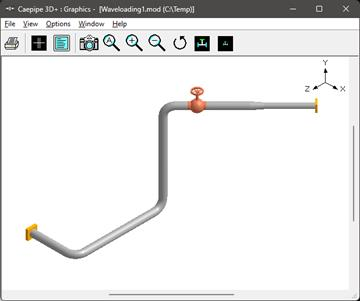
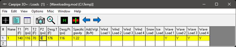
Step 1 (Layout and Graphics Windows):

Snapshots shown below are from a sample CAEPIPE Stress layout that is used for Pipe stress analysis using Wave Loading (see the “Waveloading.mod” file). The piping code selected for this analysis is ASME B31.3 (2024).

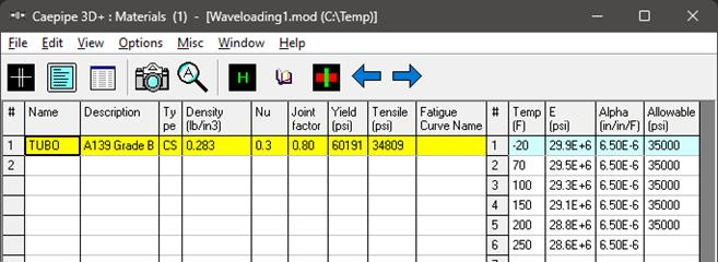
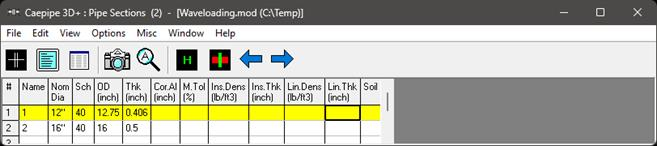
Step 2 (Materials, Sections, Loads):

Material, Section properties and Loads used for this stress layout are given below.

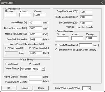
Step 3 (Waves):

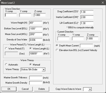
Input the Wave parameters through Layout Window > Loads > Wave 1. Select Wave Theory as “Airy’s Linear Theory”. Once all inputs are done, copy the wave data to wave 2, wave 3 and wave 4; change the wave theory in Wave 2 (through Layout Window > Loads > Wave 2) to Stokes 5^th Order Theory, in Wave 3 to Cnoidal 5^th Order Theory and in Wave 4 to “Automatic”.

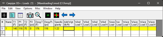
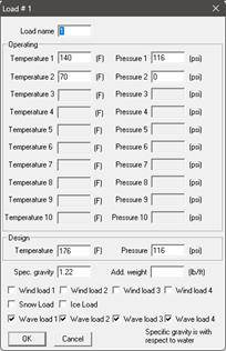
Step 4 (Loads):

Assign the defined waves to Loads by selecting Layout Window > Misc > Loads or (Ctrl + Shift+ L). Double click the Load 1 and turn on Wave load 1, Wave load 2, Wave load 3 and Wave load 4 as shown.

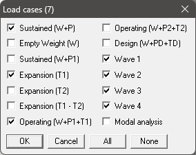
Step 5 (Load Cases):

Select Wave 1, Wave 2, Wave 3 and Wave 4 along with Sustained, Expansion 1 and Operating 1 in Load cases to be analysed through Layout Window > Loads > Load Cases… Finally, Save and Analyze.

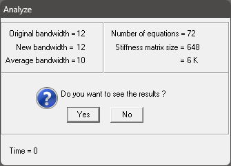
Step 6 (Results):

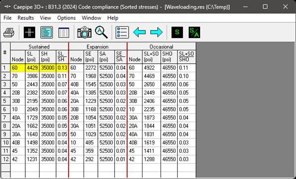
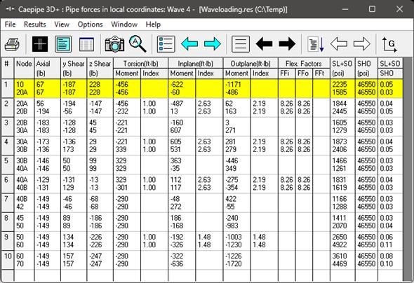
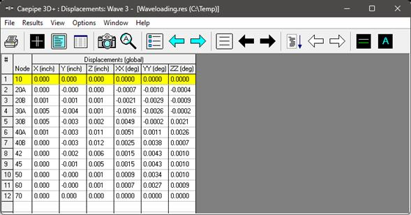
The effect of wave loading in CAEPIPE Results can be seen in Sorted stresses, Code Compliance, Elemental Forces & Moments, Support Load summary etc. As explained earlier, Forces and Moments due to Wave Loading are added in Occasional case and Buoyancy Forces are added in Sustained case. Below are a few snapshots of the Wave Loading related results reported in CAEPIPE 3D+.

Sorted Stresses, Support load Summary, Elemental Forces & Moments, Displacements

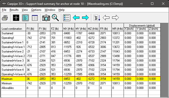
Support Loads

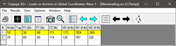
From the above support load snapshots for wave 1, wave 2, wave 3 and wave 4, the following observations can be made:

Based on the input wave parameters, “Automatic” wave selection correctly chose the wave theory as “Cnoidal 5^th Order theory” for this case (Results of Wave 3 and Wave 4 are identical).

The Forces and Moments at Anchor Node 70 are tabulated below. In the table, FR and MR are the resultant Force and Resultant Moment calculated as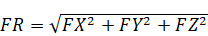

and

At Anchor Node 70
Case	Wave Theory	FX	FY	FZ	FR (lb)	MX	MY	MZ	MR (ft-lb)
Wave 1	Airy	65	-65	114	146.45	128	767	226	810.95
Wave 2	Stokes 5^th Order	10	-49	169	176.26	254	1229	4	1254.90
Wave 3	Cnoidal 5^th Order	149	171	260	344.99	291	1724	641	1860.57
Wave 4	Automatic	149	171	260	344.99	291	1724	641	1860.57

From the table above, it is evident that Airy’s theory (Wave 1) predicts the lowest loads, followed by Stokes 5th order (Wave 2), while Cnoidal 5^th Order theory (Wave 3) yields the highest. Note that Wave 4 (automatic selection) produces results identical to Wave 3, as it internally selects the most appropriate wave theory — which, in this case, is Cnoidal 5^th Order theory.

Conclusion:

CAEPIPE 3D+ has correctly selected the appropriate wave theory to be Cnoidal 5^th Order for this case and a quantitative comparison of Airy’s, Stokes 5^th order, Cnoidal 5^th Order theories has been carried out for the given layout.