Tutorial for Slug Flow Analysis using CAEPIPE

General

Slug flow is a two-phase flow pattern commonly observed in multiphase systems, such as pipelines or vessels, where both gas and liquid phases are present. In slug flow, elongated packets or "slugs" of one phase alternate with packets of the other phase flowing through the system. These slugs can vary in length and velocity, and they are separated by regions where the two phases are more evenly mixed, known as the "slug interface" or "slug front." The word slug usually refers to the heavier, slower moving fluid, but can also be used to refer to the bubbles of the lighter fluid.

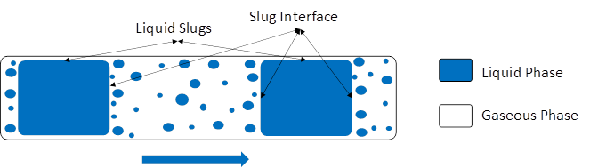
Fig 1. Schematic of slug flow showing liquid slug pushing the elongated bubbles in a pipe

In a piping system, when liquid slugs directly impact bends and T-junctions, the system will likely exhibit dynamic behaviour. Fig. 2 illustrates the schematic of slugs flowing through a bend in a piping system, highlighting the forces exerted on the bends by these slugs. These forces can influence the structural integrity and performance of the piping system, requiring careful consideration and design to mitigate any potential issues.

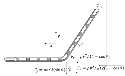
Fig 2. Slug flow through a bend and the forces caused by the slug flow on the pipe bend

Sample Problem

Problem Definition

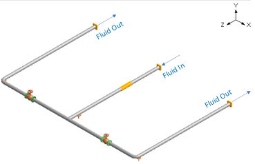
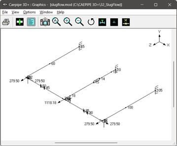
Fig 3. Layout of the Sample Problem

In the piping system illustrated in Fig.3, the 2-phase Flow direction is as shown. Within this system, slug formation occurs, as shown in Fig.4, where the force-time response at Tee is depicted. The average velocity and fluid density of the working fluid is given as 3.141 m/s and 1000 kg/m³ respectively. Also, the pipe section with bends and an equal Tee has a nominal diameter of 65 mm with a thickness of 3 mm and a bend angle of 90 degrees.

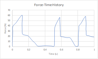
Fig 4. Slug Forces acting on the Tee of the sample piping system [3]

Preliminary Analysis:

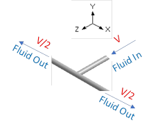
The fluid coming at a velocity (V) will be diverted into two symmetric streams at the T-junction. For the same pipe cross-section, applying momentum and mass balance at the T-junction results in a final velocity of (V/2) in both the opposite directions as shown below. The forces acting in Z and X directions at the T-junction and the 2 bends are as follows (Refer to Appendix A for details on derivation of slug force on a bend).

(Refer to [2])

At Tee- Node:

At Bend Intermediate Nodes:

= (1/4^th) of

at Tee node.

= (1/4^th) of

at Tee node.

We have three options to analyse this slug problem. Find below the tutorial for implementing all the three options in the same model. The 3 methods are as follows (Refer to Appendix B for further details):

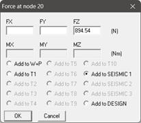
· Static loading with DLF: Slug Forces (

) given above multiplied by an appropriate DLF are applied in the respective directions at the Tee and both the bend nodes. This is implemented by activating the “Static Seismic 1” with a minimal (0.001 g) g force. The steps to apply this option can be seen in the “Force” section of the CAEPIPE Technical Reference Manual [2]. For illustrative purpose, a DLF value of 2.0 is chosen for the present analysis.

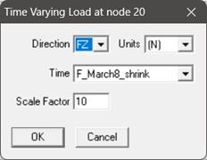
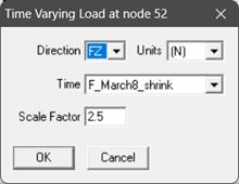
· Time History Method: Actual slug force as a function of time (Force-Time History) (See Fig. 4) is applied at the Tee and a 1/4^th of it is applied at bend intermediate nodes. This time history analysis is turned ON by activating the “Time history” in load cases. The steps to input the relevant data can be seen in the sections titled “Time functions” and “Time History Load” in CAEPIPE User’s Manual [1]

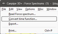
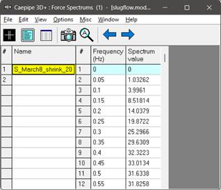
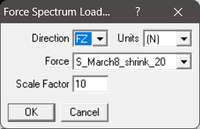
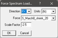
· Force Spectrum Method: The Force-Time History is converted to a force spectrum (See Fig. 5) using in-built CAEPIPE option “Convert time function” and applied at the Tee and 1/4^th of it is applied at bend intermediate nodes. This force spectrum analysis is turned ON by activating the “Force Spectrum” in load cases. The steps to input the relevant data can be seen in “Force Spectrum” section of the CAEPIPE Technical Reference Manual [2]. Fig. 5 shows the Force Spectrum as converted by CAEPIPE. Cutoff frequency of 20 Hz and number of modes of 20 are chosen for this conversion.

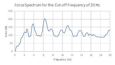
Fig 5. Force Spectrum at the Tee generated by CAEPIPE for the Force-Time History shown in Fig.4.

NOTE 1: The values provided in this tutorial are for illustrative purposes only and are used to show the procedure to perform the slug flow analysis using CAEPIPE. Users are required to input the actual values relevant to their specific cases.

NOTE 2: As stated in the Section titled “Force Spectrum” in CAEPIPE Technical Reference Manual [2], CAEPIPE uses the force spectral value corresponding to the maximum input frequency even for all natural frequencies beyond the maximum input frequency. Similarly, CAEPIPE uses the force spectral value corresponding to the minimum input frequency for all frequencies below the minimum input frequency. In view of the above, in order not to use the spectral values beyond 20 Hz for this sample problem, we have manually input the force spectral value of zero for 20.05 Hz in the Force Spectrum generated.

INPUT

Attached is a sample CAEPIPE model for Slug Flow System as shown in Fig. 3. Since the actual slug forces acting on the Tee and bend are small, the actual forces are multiplied by a factor of 10 in all the methods to get a discernible support loads at the anchors. Below are the snapshots from the model.

Step 1

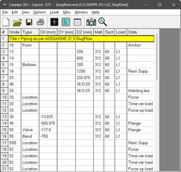
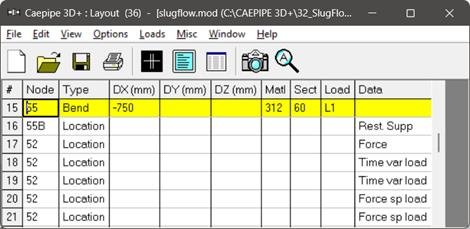
The layout window and graphics window are input as shown below. The Analysis type and Analysis options can be seen through Layout window > Options.

Step 2

The material properties, pipe sections, and loads can be seen through Materials, Sections and Loads options respectively from Layout window > Misc.

Step 3

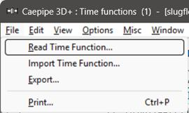
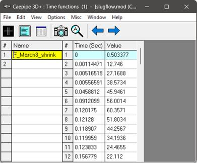
The Force-Time history as an ASCII file attached with the tutorial zip file named “SlugFlowLoad.txt” is read into CAEPIPE as described in the section titled “Time functions” in the CAEPIPE User’s Manual [1]. Import this ASCII file into CAEPIPE through Layout window > Misc > Time Functions > File > Read Time Functions.

Step 4

Force-Spectrum for the above Force-Time function is then generated using CAEPIPE as explained in the section titled “Force Spectrum” in the CAEPIPE Technical Reference Manual [2]. The obtained spectrum is shown in Fig. 5. Convert the time-history to Force spectrum in CAEPIPE through Layout window > Misc > Force spectrums > File > Convert time function.

Step 5

Apply the ‘Force’ card, ‘Time-History’ card and ‘Force Spectrum’ card as explained above and as shown below at the T-Node 20.

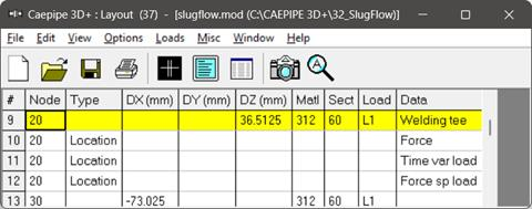
Step 6

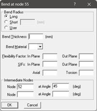
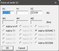
Apply the ‘Force’ card, ‘Time-History’ card and ‘Force Spectrum’ card as explained above and as shown below at the intermediate bend node 52.

Step 7

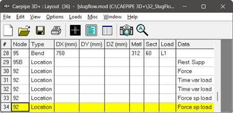
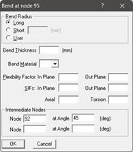
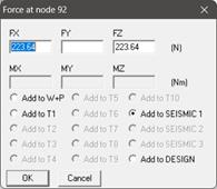
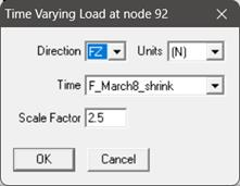
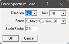
Similarly, apply the ‘Force’ card, ‘Time-History’ card and ‘Force Spectrum’ card as explained above and as shown below at the intermediate bend node 92.

Step 8

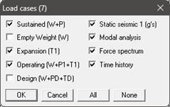
Load the cases as shown below. Save the model and perform the analysis through Layout window > File > Analyze. CAEPIPE will apply these loads to compute the response of the piping system by performing a Time history analysis, Force-spectrum analysis, Static seismic 1 analysis along with other load cases specified for the piping system.

RESULTS

Step 9

Upon successful analysis, CAEPIPE will now show “Time history”, “Frequencies”, “Dynamic susceptibility” among others as shown.

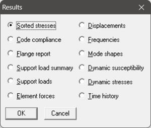
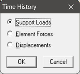
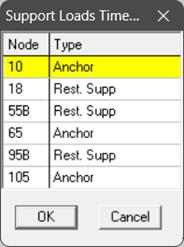
For time history results, you are shown the following dialog box (left) from which you need to select an item of interest. Then, you are shown a list of supports in the model as shown in right.

Similarly, the snapshots of all the other results are shown below.

Step 10

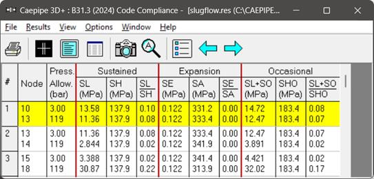
In the above snapshot, the Occasional (SO) stresses are the maximum of the Occasional (SO) stresses computed for Static Seismic load, Time-Varying load, Force Spectrum load at every individual node.

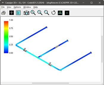
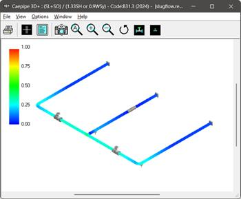
Fig 9. Stress contours of the model (SL on the Left and SL+SO to the right).

Step 11 (Support Loads, Modes, and Mode shapes)

Static Seismic 1

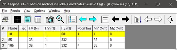
Fig 6. Anchor Loads (Static Seismic 1).

For the Static Seismic case, the static slug forces applied at T-node 20, and intermediate bend nodes 52 and 92 (894.54 N, 223.64 N, and 223.64 N in the Z-direction) are mostly transmitted to anchor nodes 10, 65, and 105 in the Z-direction, resulting in support loads of 681 N, 332 N, and 332 N. This is because, in static analysis, any externally applied force is always transmitted to the stiffer regions of the structure, which, in this case, are the anchors at nodes 10, 65, and 105 for the Z-direction. However, for the X-direction, the applied forces of 223.64 N and -223.64 N at intermediate bend nodes 92 and 52 cancel out, resulting in very small support loads (1 N, 36 N, and 36 N) at the anchors (nodes 10, 65, and 105).

Finally, there is no force applied in the vertical (Y-direction), and hence the support loads in the Y-direction at the support nodes are also almost zero. The observations in the Y-direction are disregarded from this point forward.

Dynamic Cases (Force Spectrum and Time History)

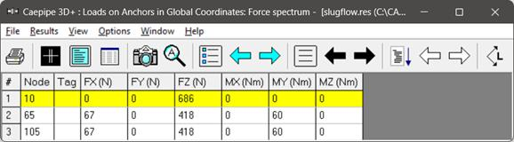
Fig 7. Anchor Loads (Force Spectrum).

Fig 8. Anchor Loads (Time History).

In dynamic analysis options such as Force Spectrum and Time History, forces are not directly transferred to the support nodes but are influenced by the natural modes of vibration of the system. For instance, in Fig. 7 and 8, the Z-direction support loads can be seen as 686 N, 418 N, and 418 N for the Force Spectrum case and 301 N, 183 N, and 183 N in the Time History method. This distribution of forces in both cases is due to the presence of a dominant vibration mode in the Z-direction (Mode 2 at 9.464 Hz in Fig. 9) that aligns with one of the peaks of applied dynamic forces, as indicated in the Force Spectrum plot of the applied load in Fig. 5. Consequently, the applied dynamic load gets distributed to the supports through the first dominant mode in Z-direction (Mode 2). Refer to Fig. 10 to observe that all the support nodes are active in Mode 2, and hence, the applied dynamic force gets distributed to these support nodes based on their participation.

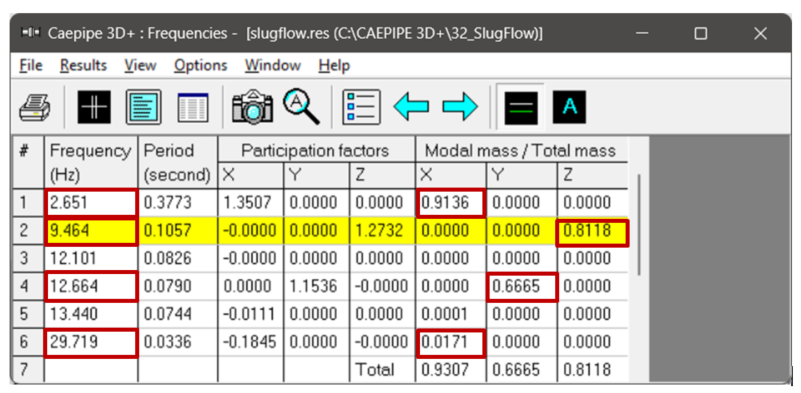
Fig 9. Frequencies result from CAEPIPE showing the dominant modes and the respective directional participation factors.

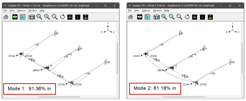
Fig 10. Mode shapes for the dominant Modes 1 & 2 in X and Z directions.

Similar to the static case, for X-directional support loads, the applied forces cancel out even in dynamic cases, resulting in minimal loads in X-direction at support anchors.

Lastly, from the support loads snapshots (Fig. 7 & Fig. 8), it can be observed that the force spectrum method results in higher support loads than the time history method.

Conclusions

From the above analysis, it can be seen that

· The time history method proves to be realistic, while the force spectrum method is more conservative.

· The Static loading with DLF method is the simplest to apply and the resulting support load results get directly influenced by the assumed DLF factor.

· Therefore, Time history method is always preferred over Static loading method with DLF (or) Force spectrum method. The Force-Time history can be obtained using CFD simulations or experimental observations.

· Dynamic analysis reveals that the system's response is influenced by natural modes of vibration, leading to distinct load distributions compared to static analysis. Understanding these differences is critical for precise support load predictions and ensuring piping system integrity and safety.

References

[1]. SST Systems, Inc., CAEPIPE User’s Manual. Retrieved from https://www.sstusa.com/pdf-download.php?id=3

[2]. SST Systems, Inc., CAEPIPE Technical Manual. Retrieved from https://www.sstusa.com/pdf-download.php?id=4

[3]. Klinkenberg, A. M., & Tijsseling, A. S. (2021). Stochastic mechanistic modelling of two-phase slug flow forces on bends in horizontal piping. International Journal of Multiphase Flow, 144, 103778. ISSN 0301-9322. Retrieved from https://www.win.tue.nl/~atijssel/pdf_files/Klinkenberg-Tijsseling_2021.pdf.

Appendix A - Slug Flow Force on Bends

Derivation

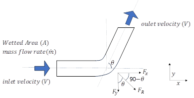
Fig A1. Schematic showing force due to slug flow along any bend

For the case shown in Fig.A1, liquid with a density of

is flowing in a pipe of Diameter ‘

and wetted area ‘

with a mass flow rate of ‘

and inlet velocity of ‘

. The bend angle is ‘

radians.

Net force acting in x-direction:

Net Force acting on the bend in x-direction is ‘

= Rate of change of momentum in x-direction

Net force acting in y-direction:

Net Force acting on the bend in y-direction is ‘

= Rate of change of momentum in y-direction

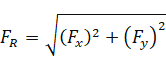
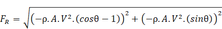
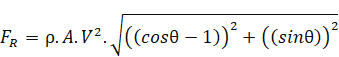
Net Resultant force acting on the bend:

Resultant Force acting on bend ‘

The resultant force

acts at an angle

with the upstream direction as shown in Fig. A1. This is the net resultant force experienced by the bend.

Appendix B - Slug Flow Analysis Options using CAEPIPE

There are three ways to analyse a piping layout with slug flow using CAEPIPE as detailed below.

Option 1: Simplified Analysis - Static Force Method

Given below are the steps for applying the Slug Flow load as a Static Force using CAEPIPE.

Step 1: Compute the Maximum Reaction Force in the three Global directions (FX, FY and FZ) from the Slug Flow characteristic from any of the available CFD tools or solvers.

Step 2: Multiply the Maximum Reaction Force with a Dynamic Load Factor (DLF) to arrive at a Static Force equivalent to a dynamic Slug force.

Step 3: Generally, the Stresses due to Slug Flow are evaluated under Occasional Load. Hence, to include the Static Force computed in Step 2 above as part of Occasional Load case, input a small g-factor (say 0.001) in global X, Y and Z directions in CAEPIPE through Layout Window > Loads > Static Seismic 1.

Step 4: Apply the force computed in Step 2 at all nodes where the flow changes its direction (such as at Bends, Tees, etc.) using a “Force” Data Type available in CAEPIPE by specifying the Forces in Global X, Y and Z directions and by selecting the option “Add to Seismic 1”.

When done, turn on the Load Case “Static Seismic 1” through Layout Window > Load Cases and perform the analysis. CAEPIPE will show the Displacements, Forces and Moments and Support Loads results under “Static Seismic 1” and Code Compliance and Sorted Stresses under Occasional Load.

Option 2: Detailed Analysis - Time History Method

Step 1: Time History Method is used when you have the actual time varying slug force function (See Fig.B1 for a sample slug force as a function of time). This can be obtained either by conducting experiments or from CFD simulations.

Step 2: Once a Force-Time Function is available, Input the Time Functions (Force as a function of time) in different directions in CAEPIPE through Layout Window > Misc > Time functions. For further details on performing the Time History Analysis using CAEPIPE, see the sections titled “Time functions” and “Time History Load” in CAEPIPE User’s Manual (See Reference [1] given above).

Step 3: Use the “Time var load” Data type in CAEPIPE to apply force as a function of time at all nodes where the flow changes its direction (such as at Bends, Tees, etc.) in Global X, Y and Z directions. You can use the element type “Location” in CAEPIPE to define more than one “Time var load” at the same node.

When done, turn on the Load Case “Time history” through Layout Window > Load Cases and perform the analysis. CAEPIPE will show the Displacements, Forces and Moments and Support Loads results under “Time history” and Code Compliance and Sorted Stresses under Occasional Loads.

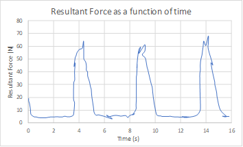
Fig B1. Sample time history of slug force amplitude observed at the bends of a piping layout.

Option 3: Detailed Analysis - Force Spectrum Method

Given below are the Steps in performing the Slug Flow Analysis using Force Spectrum Method where the Slug Flow Force is applied as a function of Frequency.

Step 1: Follow Steps 1 and 2 given under Time History Method (Option 2).

Step 2: Convert the Time Functions for Global X, Y and Z directions to the corresponding Force Spectrums in Global X, Y and Z directions in CAEPIPE through Layout Window > Misc > Force Spectrum > File > Convert Time Function by inputting the required parameters. Given below is a snapshot (Fig. B2) for converting the Time History data shown in Fig. B1 to Force Spectrum.

Step 3: The time function data for the Global Z direction is used to generate the Force Spectrum for the Global Z direction. Determining the maximum frequency, number of frequencies, and damping requires consideration of the Force time history data and the Nyquist Criteria. From Fig.B1, the time period (elapsed time between 2 successive peaks in the Force Time history) is observed to be 5 seconds, implying a frequency (1/Time period) of 0.2 Hz for the applied force. Following the Nyquist criteria, the frequency step size should be 0.2/10 = 0.02 Hz. Thus, a maximum frequency of 10 Hz (assuming all dominant force peaks occur below 10 Hz) and a number of frequencies of 500 are chosen to achieve the required step size of 0.02 Hz (=10 Hz /500). A damping percentage of 1% can be considered for this sample analysis.

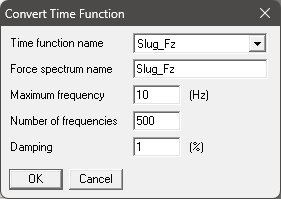
Fig B2. Snapshot of CAEPIPE input field for converting force-time function to force spectrum

For further details on performing the Force Spectrum Analysis using CAEPIPE, see the section titled “Force Spectrum” in the CAEPPIPE Technical Reference Manual (See Reference [2] above).

Use the “Force Sp load” Data type in CAEPIPE to apply force as a function of frequency at all nodes where the flow changes its direction (such as at Bends, Tees, etc.) in Global X, Y and Z directions. You can use the element type “Location” in CAEPIPE to define more than one “Force Sp load” at the same node. After inputting the required data, turn on the Load Case “Force Spectrum” through Layout Window > Load Cases and perform the analysis. CAEPIPE will show the Displacements, Forces and Moments and Support Loads results under “Force Spectrum” and Code Compliance and Sorted Stresses under Occasional Loads.

Among the above three (3) options, in general, Option 1 (Static Force Method) is the simplest to apply. Option 2 (Time-History Method) is the most realistic. Option 3 (Force Spectrum Method) is more conservative than Option 2 but not as realistic as Option 2.